Maps to: MIT 6.S978 Deep Generative Models (Fall 2024), Reading · Tue 10/29/2024 · Discrete Diffusion (student paper session). Required papers:
- J. Austin, D. D. Johnson, J. Ho, D. Tarlow, R. van den Berg, Structured Denoising Diffusion Models in Discrete State-Spaces (D3PM), NeurIPS 2021;
- S. Gong, M. Li, J. Feng, Z. Wu, L. Kong, DiffuSeq: Sequence to Sequence Text Generation with Diffusion Models, ICLR 2023;
- A. Lou, C. Meng, S. Ermon, Discrete Diffusion Modeling by Estimating the Ratios of the Data Distribution (SEDD), ICML 2024.
Basis: This session consisted of student presentations, with no published slides. The notes are organized around the session’s question: text has no “add Gaussian noise”, so how does diffusion work there? The three papers give three answers: corrupt tokens with Markov chains (D3PM), go back to continuous space through embeddings (DiffuSeq), and replace the score by probability ratios (SEDD). A final section (§5) adds the 2024 view that ties them together: masked diffusion as a weighted masked language model (MDLM, MD4, RADD). Paper claims are labelled “the paper reports / argues”. All experiments were designed for these notes and run on a CPU with a tiny English-like language whose probabilities are exact: a hidden Markov model, so every likelihood, conditional and probability ratio is computable. Several outcomes differed from what I expected and are reported as they came out:
- the ELBO’s own 1/t weighting trained a worse masked model than BERT’s weight 1;
- SEDD needed its implementation’s output scaling to work;
- masked diffusion stayed behind autoregression at this size;
- DiffuSeq’s task turned out to be easy.
Code:
code/lecture15/— 5 scripts + the shared modulediscrete_diffusion.py. They run in 2–130 s. Reading time: 4–5 hours including running the code.
0. How to read this lecture
0.1 Where we are
Everything so far in Unit V lived in continuous space:
- Gaussian noise (Lectures 12–13);
- blur and other degradations of continuous pixels (Lecture 14);
- Lecture 8’s tokenizer, which produced continuous latents so that a diffusion head could model them.
But language, code and VQ image tokens (Lecture 7) are discrete: a sentence is a sequence of symbols from a finite vocabulary. There is no “slightly noisier word”; there is no gradient ; there is no Gaussian.
Three answers, one per paper:
| paper | idea | noise | what is learned |
|---|---|---|---|
| D3PM | corrupt each token by a Markov chain with transition matrices | uniform resampling, [MASK], or structured | , plugged into the exact posterior |
| DiffuSeq | map words to learned vectors and use Gaussian diffusion there | Gaussian, on embeddings of the target only | (a vector), rounded to the nearest word |
| SEDD | replace the score by ratios between neighbouring sequences | uniform or [MASK], in continuous time | the “concrete score”, trained by score entropy |
0.2 Learning goals
- Define discrete forward processes by transition matrices; derive the closed form and the posterior ; compare uniform, absorbing and structured noise (§2).
- Derive D3PM’s loss: the variational bound with the -parameterization, the hybrid loss, and its absorbing special case (§2).
- Explain DiffuSeq’s partial noising, the rounding step, and the clamping trick (§3).
- Define the concrete score and the score-entropy loss; show that its denoising version is minimized by the true ratios; show that for absorbing noise the concrete score is a scaled clean conditional (§4).
- Write masked diffusion’s ELBO as a weighted masked-language-model loss; explain the trade-offs against autoregression: likelihood, parallel decoding, infilling (§5).
0.3 Map
| Section | Content | Code |
|---|---|---|
| §1 | The toy language: exact probabilities | — |
| §2 | D3PM | 01_d3pm_forward.py, 02_d3pm_grammar.py |
| §3 | DiffuSeq | 05_diffuseq.py |
| §4 | SEDD: concrete scores and score entropy | 03_concrete_score.py |
| §5 | Masked diffusion vs autoregression | 04_masked_vs_ar.py |
| §6 | The big picture | — |
1. The toy language
To grade discrete generative models we need data whose distribution we know exactly. The course’s glyphs are continuous, so this lecture adds a language: 13 words (the a big small cat cats dog dogs sees see runs run .) and a hidden Markov model over parts of speech:
The subject’s number lives in the hidden state from the determiner to the verb:
- “the big cats see” is allowed and “the big cats sees” has probability 0 — a dependency across intervening words;
- “a” only goes with singular nouns.
Sentences follow each other; a training example is the first 12 words of the stream, e.g.
the dogs see a big dog . a small dog sees the
a cat sees a small dog . a big big dog sees
What is exact.
- Likelihood. is exact by the forward algorithm.
- Entropy. The language has 0.903 nats per word (1.30 bits). No model can achieve a lower average .
- Grammaticality. A sequence is grammatical iff . Random word strings never are (0 of 100,000).
- Conditionals and ratios. The forward–backward algorithm gives every conditional , and every ratio for sequences differing in one position.
- Noised marginals. Corrupting each word independently by a channel yields another hidden Markov model, with emission matrix (emit, then corrupt; Exercise 4). So the marginals of every forward process below are exact too, with no enumeration of the sequences.
Samples are graded by four numbers:
- the fraction that is grammatical;
- −log p_data: the true language’s negative log-probability of the grammatical samples, per word. This is “generative perplexity” with the true model in place of GPT-2. The language’s own samples score 0.904; much lower means repetitive;
- the number of distinct samples out of 2000 (the language’s own: 1913);
- the model’s own likelihood bound on held-out text.
2. D3PM: diffusion with transition matrices (Austin et al.)
2.1 The forward process
Represent a token as a one-hot row vector . One forward step multiplies it by a stochastic matrix:
Each token is corrupted independently. The paper’s families (transition_matrix):
| family | where it ends | use | |
|---|---|---|---|
| uniform (Hoogeboom et al. 2021) | uniform over words | generic | |
| absorbing | all [MASK] | text (best in the paper) | |
| discretized Gaussian | transitions to nearby values more likely | ≈ uniform | ordinal data such as pixel intensities |
| nearest neighbours in embedding space | transitions to similar tokens | structured | text, “corrupt toward similar words” |
For uniform and absorbing noise the product has a closed form, with and the replacement distribution (Exercise 1). It is the discrete twin of : training needs no simulation. We use with T = 100 — D3PM’s absorbing schedule, which removes the same amount of information per step.
Code 01 checks the closed forms (product vs formula: within ) and measures what one corrupted token still says about the clean one, :
| t | ᾱ_t | absorbing | uniform | neighbour (swap within word class) |
|---|---|---|---|---|
| 0 | 1.00 | 2.395 | 2.395 | 2.395 |
| 25 | 0.75 | 1.796 | 1.352 | 1.951 |
| 50 | 0.50 | 1.198 | 0.681 | 1.716 |
| 90 | 0.10 | 0.240 | 0.044 | 1.541 |
| 100 | 0.00 | 0.000 | 0.000 | 1.533 |
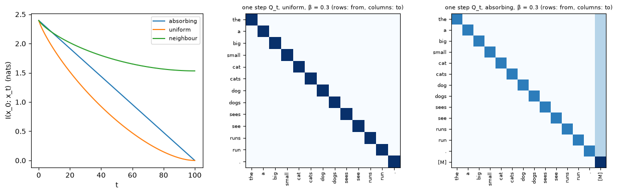
- Absorbing noise destroys information exactly linearly: . A visible token is certainly clean and a masked one says nothing, so every position knows whether it is corrupted.
- Uniform noise destroys more: a visible “cat” might be a replacement. The reverse model must also find which visible words are fake.
- The neighbour process keeps the word class forever (1.533 nats remain at t = T). Structured matrices choose what is destroyed first — the analogue of Lecture 13’s noise schedules, at the level of meaning. Its end point still depends on the data, though, so it cannot serve as a sampling prior on its own.
Where the processes end. Uniform noise ends in the uniform distribution (each word 0.077). Absorbing noise ends with every token [MASK]: one single sequence, as degenerate as Lecture 14’s total blur. The entropy of the noised language (exact, via the noised HMM) makes this vivid:
| ᾱ | absorbing | uniform |
|---|---|---|
| 1.00 | 0.903 | 0.903 |
| 0.50 | 1.319 | 2.301 |
| 0.05 | 0.301 | 2.564 |
Uniform noise drives the entropy up to . Absorbing noise first raises it (which positions are masked is random) and then drives it to 0. A sampler that starts from all-[MASK] must create all of the data’s entropy along the way. §5 shows how: every reverse step samples the revealed words. That is the difference from Lecture 14’s deterministic cold diffusion.
2.2 The posterior and the reverse step
By Bayes’ rule and the Markov property:
Code 01 checks it against 200,000 simulated chains (maximum difference 0.0012). For absorbing noise it is almost trivial. A visible token stays as it is. A [MASK] becomes with probability — here exactly — and stays masked otherwise.
The -parameterization. As in DDPM, the network does not output directly. It predicts the clean token, , at every position (a bidirectional Transformer), and the reverse step averages the true posterior over that prediction:
The paper writes this as , normalized over . That version re-weights by the likelihood of . For absorbing noise the two coincide; d3pm_reverse uses the first form. Two advantages:
- the reverse step automatically respects the structure of Q (a visible token in absorbing diffusion stays visible);
- one network serves every step, and big jumps use the same formula with , .
2.3 The loss
The variational bound is DDPM’s (Lecture 12 §4), term by term:
The KLs are between categorical distributions over 13–14 values, computed exactly. D3PM trains on a hybrid loss, : the bound plus a little direct cross-entropy on (λ = 0.01 here), which the paper reports improves training.
Absorbing noise makes the bound simple. For a masked position, puts mass on and the rest on [MASK]. The model puts on words and the same rest on [MASK]. Hence (Exercise 2)
The bound is a weighted masked-language-model loss, with weight for our schedule. Visible positions contribute nothing. §5 takes this to continuous time.
2.4 Experiment: uniform vs absorbing
Code 02 trains the same Transformer (width 64, 3 layers, 3000 steps, ~45 s) with each noise:
| noise | −ELBO (nats/word; truth 0.903) | grammatical, 100 / 25 / 10 steps | −log p_data (100 steps) | distinct |
|---|---|---|---|---|
| uniform | 1.054 | 0.637 / 0.535 / 0.369 | 0.895 | 1958 |
| absorbing | 0.959 | 0.733 / 0.611 / 0.419 | 0.900 | 1948 |
Typical absorbing samples:
a cat sees the dogs . a cat runs . the dogs
the big dog sees the small dogs run . the dogs see ← an error: two verbs- Absorbing is better on both counts, as the paper found for text: with [MASK], each corrupted position announces itself, and the model only fills blanks.
- Neither model is perfect at this budget: a quarter to a third of the samples break a rule somewhere in 12 words, though the grammatical ones are typical sentences (−log p_data ≈ 0.90, like the language’s own).
- Fewer, larger reverse steps lose grammaticality. In one big jump many positions change at once, and given they are sampled independently, so “the cats … sees” can happen. §5 measures this directly.
2.5 What the paper reports, and the connections it draws
D3PM is evaluated on character-level text (text8), on word-piece text (LM1B), and on CIFAR-10 images with the discretized-Gaussian matrix. The paper reports:
- absorbing noise is the best of its families on text;
- the discretized Gaussian works well on images, with competitive likelihoods.
It also points out two connections that became central later:
- BERT is a one-step absorbing diffusion model. It predicts masked tokens from visible ones at a single masking rate.
- An autoregressive model is an absorbing diffusion model with a deterministic order. Mask the last token, then the last two, and so on; Lecture 8’s order-agnostic AR models are the random-order version.
3. DiffuSeq: back to continuous space (Gong et al.)
3.1 The idea
Instead of inventing discrete noise, make the tokens continuous:
- map each word to a learned embedding vector;
- run the Gaussian diffusion of Lectures 12–13 on the embeddings;
- at the end, map each vector back to the nearest word (“rounding”).
This is Diffusion-LM (Li et al. 2022). DiffuSeq turns it into a sequence-to-sequence model with partial noising. The input is , but noise is applied only to the target part. The source stays clean in every and acts as the condition, seen by a single bidirectional Transformer. No encoder–decoder split and no classifier is needed.
The training objective (simplified) has three terms:
with :
- the first term is the usual -prediction loss;
- the other two are rounding losses. They are needed because the embeddings are learned jointly: without them, all embeddings could shrink to one point and make the first term trivially zero.
At sampling time the clamping trick (from Diffusion-LM) optionally replaces by the nearest word’s embedding at every step, so the trajectory cannot settle between words.
3.2 Experiment: a one-to-many task
Code 05 builds a task with both a deterministic and a free part: flip the number of the subject.
the cats see the small dog .   →   the cat sees the small dog .     or   a cat sees the small dog .
a dog runs .                   →   the dogs run .
A plural subject turned singular may take “the” or “a” (50/50 in the training targets); a singular turned plural must take “the”. The model is DiffuSeq with 16-number embeddings and a width-64, 3-layer Transformer, trained 2000 steps (38 s). It is compared with a same-size autoregressive model over [source; target]:
| model | steps | clamping | valid | “a” share (target 0.5) | both choices seen for one source |
|---|---|---|---|---|---|
| DiffuSeq | 50 | no | 1.000 | 0.545 | 1.00 |
| 50 | yes | 1.000 | 0.627 | 1.00 | |
| 10 | no | 1.000 | 0.557 | 1.00 | |
| 2 | no | 1.000 | 0.531 | 1.00 | |
| 1 | no | 1.000 | 0.709 | 0.96 | |
| AR, sampled | 8 calls | — | 0.998 | 0.470 | 1.00 |
| AR, greedy | 8 calls | — | 0.999 | 0.062 | 0.00 |
- Gaussian diffusion on embeddings solves the task. Every flip is correct and the free choice comes out near 50/50: a seq2seq model that samples answers.
- The task was easier than I planned: every configuration is 100% valid, even with one step. What differs is the free choice.
- One step biases it (0.71 “a”). A single step returns the network’s average of the “the” and “a” embeddings, and rounding picks whichever is nearer. This is Lecture 13’s “one step returns the mean” (§3.1 there), hidden by rounding.
- Clamping biases it too (0.63–0.71). Rounding at every step commits early to the currently nearest word, removing uncertainty that later steps would have resolved. On this task the trick bought nothing.
- The AR baseline is just as accurate and samples just as well. Greedy decoding returns one answer per source (“both seen” = 0). That is the diversity problem the DiffuSeq paper attributes to AR models decoded with beam search.
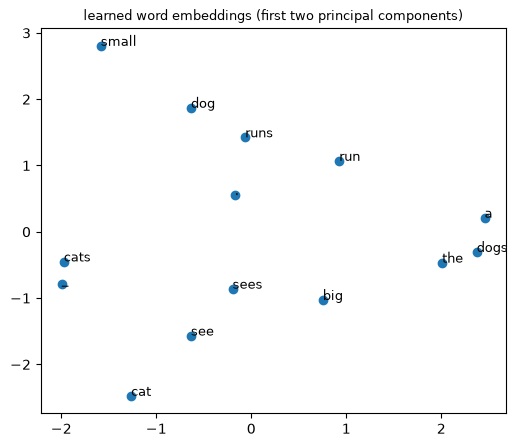
The learned embedding space is only partly interpretable. “the” and “a” — the interchangeable pair — are each other’s nearest neighbours, and see → sees, run → runs; the rest looks arbitrary at this scale. Whatever is close in embedding space is what Gaussian noise confuses cheaply, so the embedding is part of the model.
3.3 What the paper reports
DiffuSeq is evaluated on four seq2seq tasks:
- open-domain dialogue;
- question generation;
- text simplification;
- paraphrasing.
It is compared with autoregressive and non-autoregressive Transformers and fine-tuned GPT-2. The paper reports quality competitive with the AR baselines and clearly higher diversity among samples. It uses minimum-Bayes-risk selection among several samples to turn diversity into quality.
The costs are the usual ones of continuous diffusion: many network evaluations, and a rounding step that can land on the wrong word. The paper also discusses the connection to AR and to non-autoregressive models.
4. SEDD: scores for discrete data (Lou, Meng & Ermon)
4.1 The concrete score
Score-based diffusion (Lecture 12 §6–8) learns : how the log-density changes when x moves a little. Discrete x cannot move a little. The concrete score asks instead how probability changes when x moves to a neighbour — here, a sequence differing in one position:
Like the score, the ratios do not need the normalizing constant. And they suffice to run a diffusion backwards. A forward continuous-time Markov chain on sequences, with rates , has a reverse chain with rates
(Anderson’s reverse-time SDE has a discrete counterpart). So knowing the concrete score at every t is enough to generate.
Code 03, Part 1 computes exact concrete scores with forward–backward on the noised HMM. For one sentence at α = 0.5 (α = fraction of words still clean), the absorbing case gives
x_t = "the _ sees _ cats . _ _ dog _ the cat", position 1: ratio(cat) = 0.500, ratio(dog) = 0.500, ratio(the) = 0, …since “sees” forces a singular noun. Over 1000 sentences, the log10 ratios range as follows:
| noise | min | median | max | exactly 0 |
|---|---|---|---|---|
| absorbing, α = 0.5 (masked positions) | −3.84 | −0.60 | 0.00 | 77% |
| uniform, α = 0.5 (all positions, other words) | −1.15 | −0.19 | 1.15 | 0% |
| uniform, α = 0.9 | −2.07 | −1.77 | 2.07 | 0% |
- Absorbing ratios are either exactly 0 (words the grammar forbids) or positive and at most 1.
- Uniform ratios are always positive — any word could have been any other — and their range grows as the noise shrinks.
Ratios live on a log scale, which is why SEDD predicts them through a log and needs a loss built for positive quantities.
A key identity for absorbing noise. Let position i be masked in . Then
because unmasking position i to v requires that the word was v (the clean conditional) and that it survived (odds α/(1 − α)) (Exercise 6). Code 03 checks it exactly: the difference is below at α = 0.2, 0.5 and 0.8, and the ratios at a masked position sum to α/(1 − α).
So for absorbing noise the concrete score is a time-independent clean conditional times a known factor. Learning it is training a masked language model, and the time input is redundant. Ou et al. (2024, “RADD”) and Sahoo et al. (2024, “MDLM”) build on exactly this.
4.2 Score entropy
How should a network be fitted to ratios? SEDD’s score entropy is
Each summand is the Bregman divergence of . It is non-negative, zero exactly at , and convex in . It treats a ratio of 0.001 and a ratio of 1000 on the same multiplicative footing, which a squared error would not. SEDD presents it as the discrete counterpart of score matching (Lecture 12 §7).
Like explicit score matching, this needs the unknown true ratios. SEDD’s denoising score entropy replaces them with ratios of the known forward kernels, conditioned on the clean :
is linear in r, so for fixed x the minimizer over is the posterior average of the target ratios. That average is exactly (Exercise 5) — the same trick as Vincent’s denoising score matching (Lecture 12 §7.2). With = the forward rates and an integral over t, becomes an upper bound on , a proper likelihood bound.
For absorbing noise with :
- the target ratio for unmasking a masked position to v is ;
- the forward rate of masking is ;
- the DSE integrand is .
4.3 Experiment: does score entropy learn the exact ratios?
Code 03, Part 2 trains SEDD (absorbing noise, the same Transformer, 3000 steps). It follows SEDD’s implementation in one important detail: the network’s output is scaled by the known factor , so that . This is preconditioning, as with EDM’s (Lecture 13 §5.2). The ratios remain free: nothing forces them to sum to .
| α | median |log s_θ − log s_exact| (allowed words) | share of s_θ on forbidden words | learned Σ_v s_θ | exact |
|---|---|---|---|---|
| 0.8 | 0.079 | 0.020 | 3.999 | 4.000 |
| 0.5 | 0.131 | 0.030 | 0.999 | 1.000 |
| 0.2 | 0.156 | 0.019 | 0.249 | 0.250 |
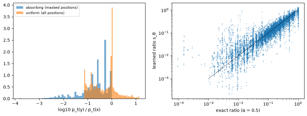
- The network learns the exact ratios. It was trained only on denoising targets, each either 0 or , yet its ratios are within ~10–15% (median), only 2–3% of its mass sits on forbidden words, and it learns the normalization to three digits.
- Its bound is the best of this lecture’s diffusion models: 0.949 nats/word, against D3PM-absorbing’s 0.959.
- Its samples are not. At 100 steps 64% are grammatical, against D3PM-absorbing’s 73%. The 2–3% left on forbidden words adds up over the 12 words a sample reveals. A good bound and good samples are related, not identical.
- The scaling matters. Without it, the network must produce ratios whose scale swings from to with t, and the loss weight reaches 1000. In development that version reached only a bound of 1.018 and 37% grammatical samples.
4.4 What the paper reports
SEDD trains GPT-2-sized models on web text. The paper reports:
- it improves substantially on earlier discrete diffusion language models in perplexity;
- it is competitive with GPT-2 at the same size;
- its samples score better generative perplexity than un-annealed GPT-2 samples;
- quality can be traded against the number of network evaluations;
- it does prompted and infilling generation in any order.
Its absorbing variant was the stronger one, consistent with D3PM and with our experiments.
5. Masked diffusion vs autoregression
5.1 Masked diffusion is a weighted masked language model
Take D3PM’s absorbing bound (§2.3) to continuous time, with a keep-probability (here ). The ELBO becomes (Exercise 3)
That is: mask each word with probability t, predict the masked words with a cross-entropy, weight by 1/t. Three groups found this in 2024: MDLM (Sahoo et al.), MD4 (Shi et al.) and RADD (Ou et al.). SEDD’s absorbing loss with normalized ratios is the same thing (Exercise 7). D3PM, SEDD and masked LMs meet here.
Sampling reverses the masking:
- going from t to s < t, each masked word is revealed with probability ;
- its value is drawn from ;
- words revealed in the same step are drawn independently of each other.
5.2 Experiment
Code 04 trains three models of the same size (width 64, 3 layers, 3000 steps, ~39 s each): an autoregressive Transformer, masked diffusion with the ELBO’s weight 1/t, and a masked model with BERT-style weight 1.
Likelihood (nats per word; the language: 0.903):
| model | value |
|---|---|
| autoregressive (exact ) | 0.909 |
| masked diffusion, weight 1/t (ELBO) | 0.947 |
| masked model, weight 1 (its ELBO) | 0.930 |
- AR is nearly perfect. It learns one conditional per position in one fixed order. The masked model must learn every conditional for every subset of visible words — a harder task for the same network — and its bound is 0.04 nats/word worse.
- The ELBO’s own weighting trained worse than weight 1, even measured by the 1/t bound (0.947 vs 0.930). I had expected the opposite. The weight 1/t gives rare, nearly complete inputs huge weights and makes the gradient noisy — Lecture 12’s experience with the DDPM ELBO weights (§4.3 there), again. The weighting that defines the bound need not be the best one to train with.
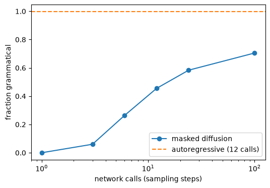
Samples (2000 each):
| sampler | network calls | grammatical | −log p_data | distinct |
|---|---|---|---|---|
| autoregressive | 12 | 0.998 | 0.906 | 1925 |
| masked diffusion | 100 | 0.705 | 0.912 | 1955 |
| 24 | 0.584 | 0.911 | 1977 | |
| 12 | 0.455 | 0.914 | 1985 | |
| 6 | 0.264 | 0.918 | 1993 | |
| 3 | 0.060 | 0.942 | 2000 | |
| 1 | 0.000 | — | 2000 |
masked, 3 calls: the small dog dog runs a big small cats run runs .- AR’s samples are almost always grammatical. Each word is drawn given all previous words, so agreement is never violated.
- Masked diffusion with 100 calls is clearly worse (0.71), reflecting its less precise conditionals.
- With fewer calls it degrades steadily: the cost of parallel decoding. Words revealed in the same step are independent given the rest, so the noun’s number and the verb’s number can disagree. At AR’s cost of 12 calls, 0.46; with 3 calls, 0.06; with 1, nothing.
This is why practical masked diffusion LMs use many steps, or confidence-based orders like MaskGIT’s (Lecture 7).
Infilling. Mask one word in the middle (positions 3–8) of 1000 sentences, and compare each model’s distribution for it with the exact conditional:
| method | calls per query | mean total-variation distance | top guess = truth |
|---|---|---|---|
| masked diffusion | 1 | 0.022 | 0.742 |
| AR + Bayes over 13 candidates | 13 | 0.005 | 0.732 |
| exact conditional | — | 0 | 0.746 |
- Both are nearly exact. In this language, the words on both sides usually pin down the missing one.
- The masked model answers in one call because this is exactly what it was trained to do.
- AR has to score every completion: 13 calls here, and for k missing words, which is hopeless for real vocabularies.
AR + Bayes is more accurate because its likelihood is. Any-order conditioning — infilling, editing, constraints on later words — is masked diffusion’s genuine advantage; exact likelihoods and cheap, consistent left-to-right sampling are AR’s.
6. The big picture
| D3PM | DiffuSeq | SEDD | masked diffusion (2024 view) | |
|---|---|---|---|---|
| state space | tokens | embeddings () | tokens | tokens |
| corruption | transition matrices | Gaussian on target embeddings | CTMC (uniform / absorbing) | masking with prob. t |
| learned object | vector | ratios | at masked positions | |
| loss | + λ CE | MSE + rounding | denoising score entropy | CE × 1/t |
| our bound (nats/word; truth 0.903) | 0.959 (absorbing) | — | 0.949 | 0.947 (0.930 with weight 1) |
| our samples | 0.733 grammatical | 1.000 valid flips (a different, easy task) | 0.642 grammatical | 0.705 grammatical (100 calls) |
The answers to the session’s question.
- Noise for discrete data is a Markov chain on tokens. Its closed forms (, the posterior, even the noised marginals of a whole sentence in our HMM) play the roles of DDPM’s Gaussian formulas.
- Absorbing ([MASK]) noise wins. It is the most informative corruption for the reverse model, because every corrupted position announces itself. With it, D3PM, SEDD and masked LMs collapse to one simple objective: a 1/t-weighted masked-LM loss.
- Lecture 14’s diversity puzzle has a discrete answer. The absorbing process ends in a single all-[MASK] sequence — as degenerate as total blur — yet generates diverse text. Each reverse step samples the revealed words from a distribution, where cold diffusion’s restorer returned one deterministic answer.
- The price is parallel decoding. Positions revealed together are independent, so masked diffusion trades steps for consistency, and at our scale it stayed behind AR in likelihood and samples. Its advantages are any-order conditioning, and generating several words per call when the words are nearly independent.
- Embedding diffusion (DiffuSeq) is the other route. It keeps the whole continuous toolkit — guidance, ODE samplers — at the price of a rounding step. Lecture 17’s discrete flow matching returns to the token-space route with the language of probability paths.
7. Summary
- D3PM. with closed-form ; the posterior ; reverse steps average it over ; train on the ELBO + λ CE. On our language, absorbing beats uniform: −ELBO 0.959 vs 1.054 nats/word, grammatical 0.73 vs 0.64.
- Absorbing noise destroys information linearly (). Its ELBO is a masked-LM loss weighted by (= 1/t in continuous time).
- DiffuSeq. Gaussian diffusion on learned embeddings, noising only the target, plus rounding. It solved a one-to-many flip task exactly with near-50/50 free choices; one step and clamping biased the choice.
- SEDD. The concrete score ; score entropy ; its denoising version is minimized by the true ratios and gives a likelihood bound. For absorbing noise, the concrete score is the clean conditional (checked exactly). Our SEDD learned ratios to ~10–15% and the best bound (0.949).
- Masked diffusion vs AR. Same objective family, different trade-offs. AR: 0.909 nats/word and 99.8% grammatical. Masked: 0.947 / 0.930 and 71% with 100 calls, 46% with 12. Infilling: masked 1 call (TV 0.022), AR 13 calls (TV 0.005).
8. Common pitfalls
- “Discrete diffusion needs a gradient-free score, so it is unrelated to score matching.” SEDD’s score entropy is a Bregman divergence that generalizes score matching, and its denoising version mirrors Vincent’s trick exactly (§4.2).
- “Uniform noise is the natural discrete Gaussian.” It is the least informative choice for the reverse model: visible tokens may be fake. Absorbing noise is what works best on text (§2.4, §4.4).
- “Masked diffusion is just BERT.” BERT trains at one masking rate with weight 1 and generates in one step. Masked diffusion trains all rates with a likelihood weighting and generates in many steps. One-step generation fails completely (§5.2).
- “More tokens per step is free speed.” Tokens revealed together are independent given the rest; consistency breaks (§5.2).
- “The ELBO weighting is the best training loss.” It defines the bound; here and in Lecture 12, a flatter weighting trained a better model, as measured by the bound itself (§5.2).
- “Embedding diffusion avoids discreteness.” It moves it to the rounding step. Rounding too early (clamping) or after one step biases the output (§3.2).
- “A degenerate end distribution means no diversity.” Not if the reverse steps sample (§2.1, §6). Lecture 14’s cold diffusion lacked diversity because its reverse steps were deterministic.
9. Exercises
Exercise 1 (closed form). Let with (rows all equal to m). Show , and that with .
Answer
. Then by induction:
For uniform noise ; for absorbing noise . (The absorbing also has its [MASK] row equal to , consistent with .)
Exercise 2 (the absorbing KL). For a masked position, show , with . What is for ?
Answer
q. It puts on and on [MASK].
p_θ. It is , which puts on each word k and on [MASK].
KL. The KL has two non-zero terms: .
The schedule. With : .
Exercise 3 (continuous time). Let be the keep-probability and take T → ∞. Show that , and that for the weight is .
Answer
With steps of size , , and the sum over steps becomes an integral. For : and .
For the cosine-like the weight is . Different schedules are different weightings of the same masked-LM losses — Lecture 13 §1.2’s lesson in discrete form.
Exercise 4 (the noised HMM). Show that if is generated by an HMM with emissions E and each token passes independently through a channel Q, then is an HMM with the same transitions and emissions .
Answer
.
The inner sum is , and the corruption of position i depends only on , which depends only on .
This is what makes log_prob(x, noised_emissions(α, kind)) exact.
Exercise 5 (denoising score entropy). Show that, for fixed and , is minimized at with , and that .
Answer
The minimizer. The objective is with . Its derivative vanishes at , and the second derivative .
Its value.
This is the discrete analogue of “the best denoiser is the conditional mean” (Lecture 12 Exercise 5).
Exercise 6 (absorbing ratios). Prove the identity of §4.1: for masked position i, .
Answer
Let be the visible positions of (other than i).
- = P(the words at are as shown and survived; the others, including i, were masked) .
- .
Divide: .
Exercise 7 (SEDD absorbing = MDLM). With , show that the DSE integrand equals . Show that this is , with equality iff .
Answer
The integrand. Substitute into . The terms cancel, leaving .
The inequality. With , we have . So , with equality iff .
Consequence. SEDD’s absorbing loss is MDLM’s loss plus a penalty for unnormalized ratios. Our SEDD learned the normalization to three digits (§4.3).
Exercise 8 (parallel decoding). In “the ___ ___ the dog .”, the two masked words are a noun and a verb that must agree in number, and each is 50/50 singular/plural. If both are revealed in the same step, independently, what is the chance they disagree? What if they are revealed in consecutive steps?
Answer
Same step. Each marginal is 50/50 and they are drawn independently, so the chance they disagree is 0.5.
Consecutive steps. The second word is drawn from , which forces agreement: 0.
Code 04’s collapse from 0.71 (100 calls) to 0.06 (3 calls) is many such pairs at once. Confidence-based orders reveal the most certain words first, which tends to reveal one member of each such pair before the other.
Exercise 9 (hands-on).
(a) In 02_d3pm_grammar.py, replace the hybrid loss by plain cross-entropy on (D3PM’s auxiliary term alone). Compare the bounds.
(b) In 04_masked_vs_ar.py, sample the masked model by revealing in each step the most confident masked positions (MaskGIT), with 12 steps. How much of the gap to AR closes?
(c) In 05_diffuseq.py, shrink the embedding size from 16 to 2 and plot the embeddings directly.
Answer (sketch)
(a) Following script 04, expect plain CE to be as good as or better than the hybrid for absorbing noise. For uniform noise the CE alone ignores the “which tokens are fake” part of the bound; expect a somewhat worse bound.
(b) Revealing confident words first resolves the agreement-carrying words (determiners, verbs) early and reduces simultaneous conflicts. Expect a large gain at 12 steps, though not AR’s 0.998.
(c) With 2 dimensions the rounding regions are easy to see: the interchangeable “the” / “a” should sit close together, and words that must never be confused far apart.
10. Further reading
Required papers
- J. Austin et al., Structured Denoising Diffusion Models in Discrete State-Spaces (D3PM), NeurIPS 2021.
- S. Gong et al., DiffuSeq: Sequence to Sequence Text Generation with Diffusion Models, ICLR 2023.
- A. Lou, C. Meng, S. Ermon, Discrete Diffusion Modeling by Estimating the Ratios of the Data Distribution (SEDD), ICML 2024.
Background and follow-ups
- E. Hoogeboom et al., Argmax Flows and Multinomial Diffusion, NeurIPS 2021 (uniform discrete diffusion).
- X. L. Li et al., Diffusion-LM Improves Controllable Text Generation, NeurIPS 2022 (embedding diffusion, rounding, clamping).
- S. Sahoo et al., Simple and Effective Masked Diffusion Language Models (MDLM), NeurIPS 2024.
- J. Shi et al., Simplified and Generalized Masked Diffusion for Discrete Data (MD4), NeurIPS 2024.
- J. Ou et al., Your Absorbing Discrete Diffusion Secretly Models the Conditional Distributions of Clean Data (RADD), 2024.
- A. Campbell et al., A Continuous Time Framework for Discrete Denoising Models, NeurIPS 2022 (CTMCs, τ-leaping).
- MIT6.S184 Lecture 6 (in Chinese): discrete diffusion from the CTMC angle.
Related notes in this course
- Lecture 5 (autoregression); Lecture 7 (VQ tokens, MaskGIT); Lecture 8 §4 (order-agnostic AR as absorbing diffusion); Lecture 12 §7 (denoising score matching); Lecture 14 §1 (degenerate end points).
11. Next lecture
Lecture 16: Flow matching (reading session · 10/31).
Lectures 12–15 all built generative models by corrupting data and learning to undo the corruption. Flow matching starts from the other end. Choose a path of distributions from noise to data — for example, straight lines between a noise sample and a data sample, InDI’s construction from Lecture 14 with y replaced by noise. Then regress the velocity field that moves samples along it. Diffusion turns out to be one choice of path among many; straight paths give simpler, faster samplers. Problem Set 5 builds conditional flow matching from scratch.