Maps to: MIT 6.S978 Deep Generative Models (Fall 2024), Reading · Tue 10/01/2024 · AR and Diffusion (student paper session). Required papers:
- T. Li, Y. Tian, H. Li, M. Deng, K. He, Autoregressive Image Generation without Vector Quantization (MAR), NeurIPS 2024;
- C. Zhou et al., Transfusion: Predict the Next Token and Diffuse Images with One Multi-Modal Model, 2024;
- J. Xie et al., Show-o: One Single Transformer to Unify Multimodal Understanding and Generation, 2024.
Optional:
- E. Hoogeboom et al., Autoregressive Diffusion Models (ARDM), ICLR 2022;
- B. Chen et al., Diffusion Forcing: Next-token Prediction Meets Full-Sequence Diffusion, NeurIPS 2024.
Basis: This session consisted of student presentations, with no published slides. These notes are organized around two questions the papers share: “must autoregression use discrete tokens?” and “can one model both predict the next token and do diffusion?” Numbers from the papers are labelled “the paper reports” and given only where the claim is central. Diffusion is a preview here. The papers rely on diffusion models, which Lecture 12 derives properly. §1 gives the one page of diffusion this lecture needs; come back after Lecture 12 for the full picture. All experiments were designed for these notes and run on a CPU with GlyphWorld images, Lecture 5’s noisy sinusoids and a 2-D toy. Several outcomes contradicted my plan and are reported as they came out:
- masked autoregression lost to raster order at our training budget;
- a Transfusion-vs-Show-o comparison flipped with the training mix;
- Diffusion Forcing needed a change to its training noise levels to work at all here, and its stabilization trick did not help.
Code:
code/lecture08/— 6 scripts + the shared modulear_diffusion.py. They run in 1–2 minutes each. Reading time: 4–5 hours including running the code.
0. How to read this lecture
0.1 Where we are
Lectures 5–7 built autoregressive models on discrete units: binarized pixels, characters, or the codes of a VQ tokenizer. A discrete unit has a convenient property: a softmax over K values can represent any distribution over them, and its cross-entropy is an exact likelihood. That is why every autoregressive image model of Lecture 7 first quantized the image.
But quantization has costs, and Lecture 7 measured them:
- information is lost (the tokenizer’s ceiling);
- codebooks collapse (dead codes) and need tricks (restarts, entropy losses);
- larger vocabularies make the prior’s job harder.
Meanwhile, diffusion models (Lecture 12) generate continuous data very well without any quantization. This session’s papers bring the two together:
| paper | what it combines |
|---|---|
| MAR | autoregression over continuous tokens; each token’s conditional distribution is a small diffusion model (“diffusion loss”); masked, random-order generation |
| Transfusion | one Transformer, next-token prediction for text and diffusion for images |
| Show-o | one Transformer, next-token prediction for text and discrete masked prediction for images |
| ARDM (optional) | order-agnostic autoregression = a discrete diffusion model |
| Diffusion Forcing (optional) | every token of a sequence has its own noise level: next-token and full-sequence diffusion as two ends of one model |
0.2 Learning goals
- State the minimal diffusion facts this lecture uses (§1): the noising formula, the noise-prediction loss, reverse sampling, temperature.
- Explain why a regression head or a Gaussian head fails for multimodal continuous tokens, and how MAR’s diffusion loss represents an arbitrary conditional distribution.
- Describe masked autoregression: random orders, several tokens per step, bidirectional attention; and what predicting several tokens at once costs.
- Explain how Transfusion and Show-o put text and images in one Transformer: the attention mask, the two losses, generation and understanding with one set of weights.
- Relate ARDM to absorbing discrete diffusion, and Diffusion Forcing to both next-token prediction and full-sequence diffusion.
- Read the experiments critically: which results are mechanisms we reproduce, and which are scale effects we do not.
0.3 Map
| Section | Content | Code |
|---|---|---|
| §1 | Diffusion in one page | ar_diffusion.py |
| §2 | MAR (1): the diffusion loss for continuous tokens | 01_heads_2d.py, 02_continuous_tokens.py |
| §3 | MAR (2): masked autoregression | 03_masked_ar.py |
| §4 | Transfusion | 04_transfusion.py |
| §5 | Show-o | 05_show_o.py |
| §6 | ARDM and Diffusion Forcing | 06_diffusion_forcing.py |
| §7 | The big picture | — |
0.4 Data and metrics
-
Glyphs. Gray GlyphWorld images: 20,000 for training (seed 700), 2,000 for testing (seed 701), scored by Lecture 3’s Judge.
metric real glyphs recognizable 1.000 valid 0.989 class entropy 3.32 bits mini FID 1.1 (0.60 for the 2000 test glyphs) nearest-real distance 0.064 -
Captions (§4–5) are three words derived from the true factors: the digit, a slant bin (left / upright / right) and a thickness bin (thin / bold). Slant and thickness are uniform in GlyphWorld, so the bins are equally likely.
-
Sequences (§6) are Lecture 5’s noisy sinusoids, 48 steps.
-
A 2-D toy (§2.3) has a known conditional distribution with three modes.
1. Diffusion in one page
Lecture 12 derives all of this; here are just the facts the papers use.
Forward process (adding noise). Take a clean vector (a token, an image, anything continuous). For a noise level :
where falls from ≈ 1 (clean) to ≈ 0 (pure noise). We use the cosine schedule with T = 1000 (for tokens) or 100 (for sequences). No simulation is needed: any noise level is one formula away.
Training (predict the noise). A network , given the noisy vector, the level and any condition c, is trained with
This is a plain regression, but its target is the noise, not the data. Different noise draws ask the network about different points of space, and together they teach it the whole distribution of given c — not just its mean.
Sampling (walk back). Start from pure noise . At each step, predict ε, estimate , and draw (s < t) from the Gaussian , whose mean and variance are known in closed form (ddpm_sample in the code). Using all T levels gives DDPM; using a subsequence takes bigger jumps.
Two knobs that matter in this lecture:
- Temperature τ. Multiply the noise injected at each step by τ < 1, and samples concentrate on high-density regions: fewer odd samples, less diversity. MAR uses this.
- Number of steps. Fewer steps are faster but approximate. We will see that, with DDPM’s per-step variance, fewer steps act like a lower temperature (§2.4).
Why is this a good way to represent a distribution? Because nothing in it assumes a shape: no number of modes, no grid, no Gaussian. That is exactly what MAR needs.
2. MAR (1): the diffusion loss
2.1 The problem: a conditional distribution for a continuous token
An autoregressive model needs, at every step, the distribution of the next token given the past. The backbone (a Transformer) summarizes the past into a vector z. A head turns z into a distribution.
| head | distribution it can represent | what goes wrong |
|---|---|---|
| softmax over a codebook (Lecture 7) | any distribution over K codes | needs a quantizer: lossy, dead codes, vocabulary trade-off |
| regression (squared error) | a single point: the conditional mean | multimodal conditionals average to a point that may look like no data (Lecture 1’s “ghosts”) |
| one Gaussian | one mode with a spread | modes are merged into one blob |
| a mixture of K Gaussians | K blobs | K must be chosen, and every mode must be roughly Gaussian |
| diffusion head (MAR) | anything | slower sampling, no exact likelihood |
MAR’s observation: the softmax was never essential to autoregression. What is essential is some way to represent and sample . A diffusion model can do that for continuous .
2.2 The diffusion loss
For each token position i, the Transformer outputs . A small MLP is trained with
and the gradient flows back through into the Transformer. The Transformer learns to produce a that makes the head’s denoising easy; the head learns the distribution given .
Details MAR uses, and which our code copies at small scale:
- The head. A few residual MLP blocks whose LayerNorms are modulated by (time embedding + ) — adaLN, the conditioning of DiT. The paper’s head is small compared with the Transformer.
- The diffusion batch multiplier. Each pair is noised several times per training step (4 in MAR and in our code). The Transformer runs once and the cheap head runs several times, which reduces the variance of the loss.
- Sampling. For each token, run the reverse diffusion with (100 steps in MAR), with a temperature τ.
- Tokens. MAR uses a continuous KL-regularized tokenizer, the kind latent diffusion uses: an autoencoder whose latent is pulled weakly toward N(0, I), with no quantizer.
2.3 Experiment: seven heads on a three-mode conditional
Code 01 replaces the past with a scalar context c and the token with a point x ∈ R². Given c, x is one of three points on the unit circle (at angles 2π(c + k/3)) plus noise of std 0.06. The conditional mean is the centre of the circle, at distance 1 from every mode. A small MLP backbone produces z from c; each head is trained for 3000 steps.
| head | test NLL (nats) | distance to nearest mode | on a mode | mode entropy (bits) | train time |
|---|---|---|---|---|---|
| true conditional | −1.693 | 0.075 | 0.997 | 1.585 | — |
| regression | — | 0.996 | 0.000 | 0.000 | 1.7 s |
| one Gaussian | 2.152 | 0.677 | 0.043 | 1.580 | 1.7 s |
| mixture of 2 Gaussians | 0.675 | 0.429 | 0.357 | 1.054 | 2.0 s |
| mixture of 3 Gaussians | −1.408 | 0.112 | 0.914 | 1.585 | 1.9 s |
| quantize 8×8 + softmax | −0.378 | 0.198 | 0.543 | 1.585 | 1.7 s |
| quantize 32×32 + softmax | −1.479 | 0.091 | 0.973 | 1.584 | 4.0 s |
| diffusion head | — | 0.064 | 0.998 | 1.585 | 14.1 s |

- The regression head outputs the centre — one point, always, on no mode. This is Lecture 1’s ghost in its purest form.
- One Gaussian covers the modes with a single wide blob; only 4% of its samples land on a mode.
- Mixtures work only with the right number of components. Two Gaussians cover two modes and smear the third; three — exactly the true number — nearly match the truth.
- Quantize + softmax works without averaging, but pays for its cells: with 8×8 cells only 54% of samples land within 0.2 of a mode centre. In 2-D, 32×32 = 1024 classes are cheap; for a 16-dimensional token the same grid would need 32¹⁶ ≈ 10²⁴ classes. Real tokenizers quantize with a learned codebook instead, and inherit Lecture 7’s troubles.
- The diffusion head puts its samples on the three modes with balanced weights, with no number of modes to choose and no grid. Its prices: it was the slowest to train (each step noises every x four times and runs an MLP), and it gives no likelihood.
2.4 Experiment: temperature and the number of steps
The diffusion head trained above, sampled in different ways (“spread” = mean distance to the nearest mode relative to the truth’s):
| reverse steps | τ | spread vs truth | on a mode | time (10,000 samples) |
|---|---|---|---|---|
| 1000 | 1.0 | 1.00 | 0.995 | 18.2 s |
| 100 | 1.0 | 0.85 | 0.998 | 1.8 s |
| 50 | 1.0 | 0.74 | 0.999 | 0.9 s |
| 25 | 1.0 | 0.62 | 0.996 | 0.45 s |
| 10 | 1.0 | 0.69 | 0.963 | 0.18 s |
| 5 | 1.0 | 2.31 | 0.812 | 0.09 s |
| 2 | 1.0 | 17.94 | 0.249 | 0.04 s |
| 100 | 0.7 | 0.60 | 1.000 | 1.8 s |
| 100 | 0.4 | 0.37 | 1.000 | 1.9 s |
- With all 1000 steps the spread is exactly right. Fewer, bigger steps make samples tighter: DDPM injects at each step the posterior variance of the step it takes, and a big jump’s posterior variance underestimates what the many small steps it replaces would have injected in total. So a few steps act like a lower temperature.
- Below about 10 steps the sampler breaks down. With 2 steps, the first jump lands near the average of the three modes — the centre again.
- Temperature tightens each mode without changing the mode weights (the mode entropy stays 1.585). This is MAR’s τ, the continuous analogue of the softmax temperature.
2.5 Experiment: continuous tokens on glyphs
Code 02 first trains a continuous tokenizer: Lecture 3’s patch encoder outputs a mean and a log-variance for each of 16 tokens of dimension 4, and the loss is the reconstruction error + 0.01 · KL to N(0, I). Tokens are the posterior means, divided by one global scale so that their std is 1.
| tokenizer | numbers / image | RMSE | valid recon | FID recon |
|---|---|---|---|---|
| continuous, 16 × 4 | 64 | 0.0346 | 0.989 | 1.89 |
| … with N(0, 0.3²) noise added to every token | 64 | 0.0627 | 0.935 | 1.57 |
| VQ, 16 tokens × 16 codes (Lecture 7) | 16 codes | 0.0802 | 0.912 | 11.3 |
| VQ, 16 tokens × 256 codes (Lecture 7) | 16 codes | 0.0515 | 0.978 | 2.1 |
- No quantizer, better ceiling. The continuous tokens reconstruct as well as real glyphs score.
- The KL term makes the space forgiving. Even with noise of 0.3 token-std added to every token, 94% of decoded glyphs are valid. A generator whose tokens are slightly off is forgiven, which is one reason to prefer a KL-regularized tokenizer over a plain autoencoder.
Then the same causal Transformer (raster order, width 64, 2 layers, 3000 steps) with three heads:
| head | recognizable | valid | class H | FID | distinct images (of 2000) | time for 2000 samples |
|---|---|---|---|---|---|---|
| regression | 1.000 | 1.000 | 0.00 | 2073 | 1 | 1.0 s |
| Gaussian | 0.732 | 0.525 | 3.13 | 177 | 2000 | 1.0 s |
| diffusion | 0.901 | 0.859 | 3.27 | 18.5 | 2000 | 5.8 s |
| Lecture 7: discrete, 16 codes | 0.648 | 26.1 | ||||
| Lecture 7: discrete, 256 codes | 0.506 | 27.2 | ||||
| Lecture 7: 1-D tokens, K = 4 | 0.856 | 20.3 |
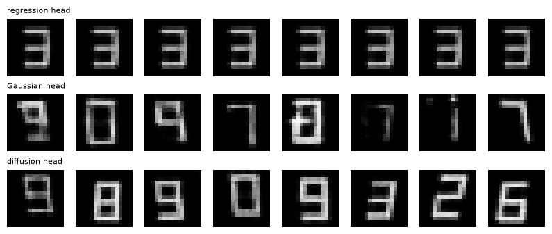
- The regression head generates one glyph, 2000 times. With no randomness anywhere, every run of 16 steps is identical. Its “valid 1.000” is a warning about metrics: one perfect image scores perfectly on per-sample quality, and the class entropy of 0 and the FID of 2073 reveal the collapse. (That the one glyph is a clean “3” rather than a blur is luck of the smooth token space: averaging happens token by token, and once the first tokens are fixed the later ones have few options.)
- The Gaussian head adds randomness but one mode per token, and blends continuations: valid 0.53.
- The diffusion head makes the same Transformer the best generator of this course so far: better than all of Lecture 7’s discrete-token models with this backbone, and level with the compact 1-D tokens. There is no codebook, no dead codes and no vocabulary trade-off. The price is 100 denoising steps of the head per token, so sampling is ~6× slower than with a one-shot head.
Developer’s note. The head’s training settings mattered. With the diffusion batch multiplier at 1 instead of 4, valid fell from 0.86 to 0.76; with 2000 steps instead of 3000, the FID rose from 18 to 39. These came from development runs, not from the scripts.
3. MAR (2): masked autoregression
3.1 From “next token” to “next set of tokens”
The chain rule holds for any order and any grouping (Lecture 5 §2):
where partition the token positions. Raster-order next-token prediction is one choice: in reading order. MAR uses another:
- a random order, freshly drawn for every image;
- groups of several tokens, so generation takes S < n steps;
- bidirectional attention: the Transformer sees all known tokens (wherever they are) plus [MASK] placeholders, and predicts the unknown ones.
This is MaskGIT’s masked generative modeling, with MAR’s diffusion head in place of MaskGIT’s softmax. MAR calls it masked autoregression and argues that it is still autoregressive: each step conditions on everything generated so far.
Training samples a random mask for every image (how many tokens to hide follows a schedule; we use MaskGIT’s cosine distribution), and the loss is computed at the masked positions only. Generation starts fully masked and reveals tokens in a random order, the number per step following a cosine schedule: few at first (when little is known), more at the end. Tokens revealed in the same step are sampled independently given what is known.
3.2 Experiment: steps, temperature, and an under-trained model
Code 03 trains a masked TokenTransformer of the same size, with the same diffusion head, for the same 3000 steps.
| generator | steps | tokens per step | valid | class H | FID | time for 2000 |
|---|---|---|---|---|---|---|
| causal, raster order (§2.5) | 16 | 1 | 0.859 | 3.27 | 18.5 | 6.0 s |
| masked, random order | 16 | 1 | 0.350 | 3.07 | 53.9 | 5.9 s |
| masked, random order | 8 | 1–3 | 0.319 | 3.07 | 55.2 | 5.4 s |
| masked, random order | 4 | 2–6 | 0.249 | 3.15 | 56.8 | 5.3 s |
| masked, random order | 2 | 5–11 | 0.130 | 3.18 | 105.5 | 5.9 s |
| masked, random order | 1 | 16 | 0.025 | 3.06 | 292.2 | 6.4 s |
Fewer steps cost quality — gradually to 4 steps, steeply below. With one step, all 16 tokens are independent given nothing: the “independent block” price of Lecture 5 §2.3. MAR (256 tokens) uses 64 steps by default, about 4 tokens per step.
The saving in time is small here, because the diffusion head dominates and runs on every token exactly once whatever the number of steps. With MAR’s large Transformer and 256 tokens, running the Transformer 64 instead of 256 times matters.
Temperature on glyphs:
| generator | valid | class H | FID |
|---|---|---|---|
| causal, τ = 1.0 | 0.859 | 3.27 | 18.5 |
| causal, τ = 0.8 | 0.897 | 3.23 | 35.5 |
| causal, τ = 0.6 | 0.926 | 3.08 | 77.8 |
| masked, τ = 1.0 | 0.350 | 3.07 | 53.9 |
| masked, τ = 0.8 | 0.533 | 2.90 | 133.1 |
| masked, τ = 0.6 | 0.709 | 2.69 | 332.1 |
Lower τ gives cleaner, more typical glyphs (higher valid rate) and a worse FID. Samples become too similar to each other, a narrower distribution than the real one, and some digits become rarer (class entropy falls). This is the fidelity / diversity trade-off of any temperature. MAR tunes τ for the best FID, which is not the cleanest-looking setting.
Why does masked lose here? The paper reports the opposite ranking at scale (bidirectional + random order beats causal + raster order in FID). Code 03 compares both models on the raster-order conditionals — the only ones the causal model knows — with the same noise levels and noises:
| position i (given tokens < i) | 0 | 1 | 2 | 4 | 8 | 12 | 15 | sum over 16 |
|---|---|---|---|---|---|---|---|---|
| causal model | 1.07 | 0.84 | 0.73 | 0.65 | 0.50 | 0.20 | 0.26 | 8.56 |
| masked model | 1.07 | 1.28 | 1.18 | 1.03 | 1.00 | 0.56 | 0.68 | 16.25 |
The masked model’s diffusion loss is about twice as high. With the same Transformer and the same 3000 steps, it has to learn the distribution of any unknown token given any subset of known ones: 16 · 2¹⁵ = 524,288 conditionals instead of 16. Each training step also scores only the masked tokens (about 10 of 16).
Masked autoregression is under-trained at our budget. In a development run, 3× more training steps raised its valid rate from 0.35 to 0.58, still below the causal model; sampling the same masked model in raster order gave 0.41, so the order is not the main problem. MAR trains for hundreds of epochs with large Transformers. The flexibility of “any order, any grouping” is paid for in training compute.
3.3 What MAR reports
- With the diffusion loss, continuous tokens beat quantized tokens with the same backbone, and the advantage holds for both causal and masked models.
- Masked autoregression with bidirectional attention beats raster-order causal autoregression.
- Its largest model reaches an FID of 1.55 on ImageNet 256×256 (with classifier-free guidance, Lecture 13), and the speed–quality trade-off is controlled by the number of autoregressive steps.
We reproduce the first point (§2.5) and the mechanism of the second, not its outcome.
4. Transfusion: next-token text and diffused images in one Transformer
4.1 Motivation
Multimodal models that both read and generate images usually take one of two routes:
- Quantize images into discrete tokens and train one language model over text and image tokens alike (Chameleon and others). Simple, but images inherit all the tokenizer’s losses (Lecture 7).
- Glue a language model to a separate diffusion model. Two models, two sets of weights.
Transfusion keeps one Transformer and gives each modality its natural loss.
4.2 Method
-
One sequence. Text tokens and image patches are interleaved in one sequence; each image is wrapped in BOI / EOI markers. Images are continuous latents (a VAE’s latent patches), projected into the Transformer’s width.
-
One mask. Attention is causal over the sequence, so text is a normal language model, but bidirectional within an image: every patch of an image sees every other patch of it.
-
Two losses. Text positions get the language-model loss (next-token cross-entropy); image positions get the diffusion loss — the whole image is noised to one level t, the time step is embedded and added to the image tokens, and the outputs predict the noise. The total is
with λ = 5 in the paper.
-
Generation. When the model emits BOI, the sampler switches to diffusion. It appends pure-noise image tokens and runs the reverse process; at every step the whole Transformer reads the text so far and predicts the noise of all image tokens. Then it emits EOI and continues with text.
-
Understanding. An image placed before text, fed clean, is read by the text positions after it.
Unlike MAR, the Transformer itself is the denoiser, and the image is generated jointly, not token by token.
4.3 Experiment: a miniature Transfusion
Code 04 trains one Transformer (width 96, 3 layers) on two layouts of 22 positions, using script 02’s continuous tokens for images:
generation   (caption first): <bos> w1 w2 w3 <boi> img_0 … img_15 <eoi>
understanding (image first) : <bos> <boi> img_0 … img_15 <eoi> w1 w2 w3
Half of the training batches use each layout (--p-und 0.5). For image-first batches the noise level is capped at t ≤ 500, so the image stays readable. The script prints the attention mask for both layouts: a lower triangle for text, a full 16×16 square block for the image.
Generation (2000 prompts; every digit equally often):
| sampler | valid | FID | digit followed | slant followed | thickness followed | time for 2000 |
|---|---|---|---|---|---|---|
| 50 denoising steps | 0.845 | 13.4 | 0.906 | 0.777 | 0.831 | 9.7 s |
| 20 denoising steps | 0.831 | 7.8 | 0.909 | 0.789 | 0.847 | 3.8 s |
| 10 denoising steps | 0.109 | 165.3 | 0.591 | 0.647 | 0.728 | 1.9 s |
| real test glyphs (the rulers’ own accuracy) | 0.989 | 0.60 | 1.000 | 0.963 | 0.894 |
“Followed” means the Judge’s classifier (digit) or a probe trained on real glyphs (slant, thickness) reads the prompted word from the generated glyph.
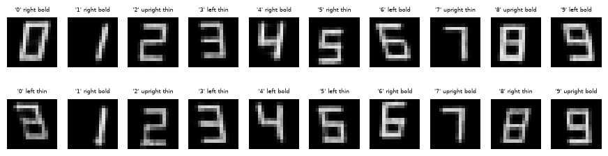
- Prompts are followed. The glyphs show the requested digit ~91% of the time; Lecture 6’s conditional PixelCNN managed 32%. Slant and thickness are followed less often than the probe can read them on real glyphs.
- 20 steps beat 50. This is §2.4’s tightening at work: fewer DDPM steps inject less noise, and this small model’s samples benefit. At 10 steps sampling breaks down.
Understanding, with the same weights (greedy decoding of the three words from 2000 real test glyphs):
| captioner | digit | slant | thickness |
|---|---|---|---|
| Transfusion | 0.994 | 0.881 | 0.823 |
| pixel probe / Judge classifier (ceiling) | 1.000 | 0.963 | 0.894 |
One set of weights generates and reads glyphs.
The training mix decides the balance. Running with --p-und 0.2 (80% caption-first batches):
| mix | valid (20 steps) | FID (20 steps) | digit followed | captions: digit / slant / thickness |
|---|---|---|---|---|
| 50% image-first (default) | 0.831 | 7.8 | 0.909 | 0.994 / 0.881 / 0.823 |
| 20% image-first | 0.942 | 2.9 | 0.992 | 0.854 / 0.507 / 0.760 |
With more generation training, generation becomes excellent — the best glyph generator in these notes so far. Captioning, however, falls apart. A small model shares its capacity between the two tasks, and the data mix decides the split.
4.4 What Transfusion reports
- Models up to 7B parameters, trained on mixed text and image data.
- The abstract’s main claim: Transfusion scales significantly better than quantizing images and training a language model over discrete image tokens (a Chameleon-style baseline), on both text-to-image and image-to-text.
- Ablations of design choices: bidirectional attention within images matters; patch encoders with U-Net down/up blocks allow larger patches, i.e. fewer image tokens; capping the noise for image-first examples helps captioning.
5. Show-o: discrete masked image modeling in one Transformer
5.1 Method
Show-o makes the other choice for images: keep them discrete.
- Image tokens. A MAGVIT-style VQ tokenizer turns the image into codes, which are added to the language model’s vocabulary.
- Image loss. MaskGIT-style masked prediction (which Show-o frames as discrete diffusion): replace a random fraction of the image codes by [MASK] and predict them with cross-entropy.
- Text loss. Ordinary next-token prediction.
- “Omni-attention”. Causal for text, full within an image — the same mask shape as Transfusion.
- Generation unmasks the image in a few parallel steps, keeping the most confident predictions each time (MaskGIT); far fewer steps than raster-order autoregression over the same tokens.
- Tasks. The paper starts from a pretrained language model and supports visual question answering, text-to-image generation, text-guided inpainting / extrapolation and mixed-modality generation with one model. Inpainting comes for free from the masked objective: mask the region, keep the rest.
5.2 Experiment: a miniature Show-o
Code 05 uses Lecture 7’s VQ grid tokenizer (16 tokens × 256 codes; reconstructions valid 0.978, FID 2.1), the same Transformer size, the same captions and the same mix as code 04.
| sampler | valid | FID | digit followed | slant followed | thickness followed | time for 2000 |
|---|---|---|---|---|---|---|
| 16 unmasking steps | 0.840 | 11.6 | 0.957 | 0.880 | 0.834 | 4.4 s |
| 8 unmasking steps | 0.746 | 10.5 | 0.945 | 0.860 | 0.820 | 2.1 s |
| 4 unmasking steps | 0.590 | 11.0 | 0.923 | 0.846 | 0.799 | 1.0 s |
Captioning with the same weights: digit 0.952, slant 0.896, thickness 0.812.
Each step is one network pass with one softmax per token, with no inner denoising loop. That makes discrete masked generation the fastest generator of the lecture. More steps help, because tokens unmasked together are sampled independently given the rest.
5.3 Transfusion vs Show-o
Same Transformer size, same data, same mix; only the image representation differs:
| mix | model | valid | FID | digit followed | time for 2000 | captions (digit / slant / thick) |
|---|---|---|---|---|---|---|
| 50% image-first | Transfusion, 20 steps | 0.831 | 7.8 | 0.909 | 3.8 s | 0.994 / 0.881 / 0.823 |
| 50% image-first | Show-o, 16 steps | 0.840 | 11.6 | 0.957 | 4.4 s | 0.952 / 0.896 / 0.812 |
| 20% image-first | Transfusion, 20 steps | 0.942 | 2.9 | 0.992 | 4.1 s | 0.854 / 0.507 / 0.760 |
| 20% image-first | Show-o, 16 steps | 0.883 | 21.9 | 0.975 | 4.5 s | 0.831 / 0.551 / 0.774 |
The comparison depends on the mix:
- With the balanced mix, neither wins outright: Transfusion has the better FID, Show-o follows the digit more often.
- With more generation training, Transfusion wins every generation column.
- Captioning is similar for both at each mix.
What does differ by design:
- Continuous tokens keep more of the image (a higher tokenizer ceiling, 0.989 vs 0.978 valid), but need an inner denoising loop.
- Discrete tokens give a cross-entropy at every position and finish in a few passes.
The papers argue from scale: Transfusion reports that its approach scales better than discrete image tokens; Show-o stresses few sampling steps and the flexibility of the masked objective.
6. ARDM and Diffusion Forcing
6.1 ARDM: order-agnostic autoregression is a discrete diffusion model
Hoogeboom et al. (2022) connect masked models and diffusion in the discrete world:
-
Order-agnostic autoregression. Train one network to predict any masked subset given the rest, as in MAR §3 or MADE’s order-agnostic training (Lecture 6).
-
The loss as a likelihood bound. Draw a step t uniformly from {1, …, D} (D = number of variables) and a random order σ. Mask the variables σ(t), …, σ(D), and score the network’s predictions at the masked positions, weighted by D/(D − t + 1):
This is an unbiased estimate of the order-averaged log-likelihood, and hence a bound on log p(x).
-
The diffusion view. This is exactly the ELBO of an absorbing-state discrete diffusion model, where “noise” replaces variables with [MASK] one at a time (Lecture 15).
-
Parallel generation. ARDMs can generate several variables per step, with a step budget distributed by dynamic programming to lose as little likelihood as possible.
MAR is the continuous-token cousin of this idea; Show-o’s masked image modeling is the discrete one.
6.2 Diffusion Forcing: every token its own noise level
Chen et al. (2024) start from sequences (video, robot trajectories) and ask how to get both the variable length and causality of next-token prediction and the guidance and long-horizon behaviour of full-sequence diffusion.
Training. Noise every token of a sequence to an independent level :
and train a causal model — the paper’s main version is an RNN, — to predict each from .
Noise as partial masking. Level K hides a token completely, level 0 shows it, and levels in between show it partially. A model trained on all combinations can then be sampled with any scheduling matrix (row m = sampling iteration, column t = token):
- token by token: past clean, current token K → 0 — next-token prediction;
- all tokens at the same level — full-sequence diffusion;
- a pyramid, where later tokens stay noisier than earlier ones.
Other claims of the paper:
- feeding generated tokens back as slightly noisy stabilizes long rollouts beyond the training horizon;
- guidance toward high-reward futures, averaged over several sampled futures (the paper’s Monte Carlo guidance), enables planning;
- results on video prediction and robot planning.
6.3 Experiment: Diffusion Forcing on noisy sinusoids
Code 06 uses Lecture 5’s noisy sinusoids (48 steps, one scalar per token) and GRUs of width 96, trained for 3000 steps. Each generated sequence is fitted with the best sinusoid. “Residual” is what the fit cannot explain (data: 0.048, the observation noise), and “ok” is the fraction with residual < 0.08.
Part 1: generation from scratch, token by token.
| model | residual | ok | amplitude (data 1.01) |
|---|---|---|---|
| data | 0.048 | 1.000 | 1.012 |
| teacher forcing, Gaussian head | 0.061 | 0.886 | 0.964 |
| Diffusion Forcing, independent levels (paper) | 0.106 | 0.042 | 0.827 |
| Diffusion Forcing, mixed levels | 0.065 | 0.898 | 0.838 |
The paper’s recipe failed at our budget. At sampling time the history is clean, but in training each token is clean with probability 1/101 and a clean stretch of history almost never occurs. The regime that matters was hardly practised in 3000 steps.
The mixed level sampler — a third of the sequences with a clean prefix, a third with one shared level, a third independent — keeps the same model, inputs and loss, and makes the sampling-time regimes common. Token-by-token sampling then matches teacher forcing. This is my modification, not the paper’s.
Part 2: one model, four schedules.
| schedule | network passes | residual | ok | amplitude |
|---|---|---|---|---|
| token by token | 48 × 100 GRU steps | 0.065 | 0.898 | 0.838 |
| pyramid, delay 10 | 570 | 0.069 | 0.824 | 0.842 |
| pyramid, delay 3 | 241 | 0.081 | 0.570 | 0.833 |
| full sequence (one shared level) | 100 | 0.214 | 0.014 | 0.593 |
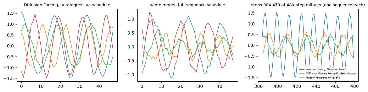
The same weights sample with any schedule, and the more the schedule staggers the tokens, the better. Full-sequence diffusion fails with a causal model, for a reason worth understanding. When all tokens are equally noisy, the correct denoiser for token t needs the noisy future tokens too: they carry information about . In score terms, the reverse process needs , which depends on . A causal model cannot see them. In a pyramid the future is noisier than the past, so it carries little information and ignoring it costs little. That is why Diffusion Forcing pairs causal models with such schedules.
Part 3: long rollouts, 480 steps (10× the training length). Mean amplitude in successive windows:
| model | amplitude at 0 → 96 → 192 → 288 → 384 | residual, last 48 | blown up (of 300) |
|---|---|---|---|
| teacher forcing | 0.95 → 0.96 → 0.99 → 1.01 → 1.04 | 0.079 | 0 |
| Diffusion Forcing, clean history | 0.84 → 0.78 → 0.70 → 0.64 → 0.60 | 0.048 | 0 |
| … history re-noised to level 3 | 0.86 → 0.77 → 0.66 → 0.57 → 0.50 | 0.047 | 3 |
- Teacher forcing keeps the amplitude (it creeps up slightly), but gets noisier.
- Diffusion Forcing keeps clean sinusoids, but their amplitude decays with every period.
- The stabilization trick made things worse here. The decay is faster, because an uncertain history pulls predictions toward the mean, and 3 of 300 rollouts blew up once the GRU state left the range seen in 48-step training.
The trick targets errors that look unlike the data, such as artifacts in generated video frames, which the model learns to clean up when it treats its own past as slightly noisy. Our errors are smooth amplitude drifts that look perfectly plausible, so there is nothing to clean. We reproduce the unification of schedules, not the stabilization.
Developer’s note. I also tried “noise as masking” for forecasting from noisy observations (σ = 0.3): feed the observed prefix as tokens at the matching noise level, ᾱ = 1/(1 + σ²). The Diffusion Forcing forecasts were worse than the teacher-forced model’s (RMSE 0.32 vs 0.28 against the clean signal), so this part was dropped from the script.
7. The big picture
7.1 Five ways to combine “sequence” and “diffusion”
| model | image tokens | loss on images | attention inside an image | generation steps (16 tokens here) | exact likelihood? |
|---|---|---|---|---|---|
| Lecture 7 AR | discrete | cross-entropy | causal | 16 | yes (of tokens) |
| MAR, causal | continuous | diffusion loss (per-token head) | causal | 16 × head’s 100 | no |
| MAR, masked | continuous | diffusion loss (per-token head) | bidirectional | 1–16 × head’s 100 | no |
| Transfusion | continuous | diffusion loss (whole image) | bidirectional | 20–50 full passes | no (text: yes) |
| Show-o | discrete | masked cross-entropy | bidirectional | 4–16 | bound only |
| Diffusion Forcing | continuous (sequence) | diffusion loss, per-token level | causal | any schedule | no |
7.2 The five components
| component | MAR | Transfusion / Show-o | Diffusion Forcing |
|---|---|---|---|
| formulation | chain rule over random groups of continuous tokens | one sequence of text and image tokens | a sequence where each token is partially masked by noise |
| representation | Transformer → z → small diffusion MLP | one Transformer, two output heads | causal RNN / Transformer |
| objective | diffusion loss per token | LM loss + λ · (diffusion or masked CE) | diffusion loss per token, independent levels |
| optimization | diffusion batch multiplier, random masks | mixing layouts and tasks | (here) mixing level patterns |
| inference | random order, cosine schedule, temperature | reverse diffusion or iterative unmasking | scheduling matrix |
7.3 Lessons from the experiments
- What a head can represent decides what a model can generate. The same Transformer went from “one image” (regression) to valid 0.86 (diffusion) by changing only the head.
- Flexibility costs training. Masked models learn many more conditionals; Diffusion Forcing learns many more noise patterns. At a fixed budget, the regime used at sampling time must be common in training.
- Unified models share capacity. The task mix changed both quality and the winner of a comparison.
- Step counts interact with variance. Fewer DDPM steps tighten samples, which sometimes helps FID (Transfusion at 20 steps) and always biases the distribution.
8. Summary
- Diffusion as a head. A small diffusion model conditioned on the Transformer’s output represents any conditional distribution of a continuous token. MAR uses it to drop vector quantization. On a three-mode toy it was the only head that matched the truth without knowing the number of modes, and on glyphs it beat every discrete-token model of Lecture 7 with the same Transformer.
- Regression heads average; Gaussian heads blur. A regression head produced one glyph 2000 times; a Gaussian head reached valid 0.53.
- Masked autoregression generates in a random order, several tokens per step, with bidirectional attention. Fewer steps cost quality (Lecture 5’s independence price). At our budget it lost to raster order because it must learn far more conditionals; MAR reports the reverse at scale.
- Transfusion puts text and continuous images in one Transformer: causal mask with bidirectional image blocks, LM loss + λ · diffusion loss. Our miniature generated the best glyphs of the notes so far (valid 0.94, FID 2.9 with 80% generation training) and also captioned.
- Show-o does the same with discrete codes and masked prediction: fastest sampling, competitive quality. The comparison with Transfusion depended on the training mix.
- ARDM shows that order-agnostic autoregression is absorbing discrete diffusion. Diffusion Forcing gives each token its own noise level, so one causal model can sample token by token, in a pyramid, or (poorly, if causal) all at once. Its stabilization trick did not reproduce on our toy.
9. Common pitfalls
- “Autoregression requires discrete tokens.” It requires a representable conditional distribution; a diffusion head provides one for continuous tokens (§2).
- “A regression head is a fine stand-in for a distribution.” It outputs the conditional mean — a ghost for multimodal conditionals and zero diversity in generation (§2.3, §2.5).
- “Valid = 1.000 means a perfect generator.” One perfect image repeated scores perfectly per sample; always check diversity (class entropy, FID, distinct samples).
- “Fewer diffusion steps only cost speed.” They also change the distribution — with DDPM’s variance, samples get tighter (§2.4).
- “Masked / random-order models are free improvements.” They learn many more conditionals and need more training (§3.2).
- “A causal model can do full-sequence diffusion.” Not well: the joint score needs the noisy future (§6.3).
- “One unified model = two models for the price of one.” The tasks share capacity, and the mix matters (§4.3).
10. Exercises
Exercise 1 (the regression head). Show that the minimizer of over functions f is . For the three-mode toy, compute , and explain the regression row of §2.3 (distance 0.996, on a mode 0).
Answer
For each z, minimize over a vector a. The gradient is , which is zero at , and the problem is convex.
For the toy, , because the three unit vectors 120° apart sum to zero.
The distance from the origin to every mode centre is 1; the learned head lands within 0.004 of the origin. No sample is within 0.2 of a centre.
Exercise 2 (classes needed by a grid head). A token has dimension d and each coordinate is cut into B cells. (a) How many classes does a softmax over cells need? (b) For d = 16 and B = 32, how does this compare with a typical VQ codebook (2¹⁴)? (c) What does a learned codebook give up compared with a grid?
Answer
(a) .
(b) , about times a codebook of 16,384.
(c) A codebook places its codes only where the data are, so few codes suffice. But it must be learned (dead codes, Lecture 7), its resolution is uneven, and any variation between codes is lost. The diffusion head avoids both the grid and the codebook.
Exercise 3 (the diffusion batch multiplier). In MAR, each is used with m different draws per training step. (a) Why does this reduce the variance of the gradient for the Transformer? (b) Why is it cheap? (c) Code 02’s development runs found valid 0.76 / 0.82 / 0.86 for m = 1 / 2 / 4. What would you expect for m = 16?
Answer
(a) The loss for one token is an expectation over (t, ε); with one draw the gradient through is a one-sample estimate of it. Averaging m draws divides the variance of that estimate by about m, so the Transformer receives a cleaner signal for the same backbone cost.
(b) The Transformer runs once per step; only the small head runs m times.
(c) Diminishing returns: once the head’s noise is small compared with the minibatch noise across images, more draws help little, and the head’s cost starts to dominate. Expect a small gain over m = 4, if any.
Exercise 4 (why fewer DDPM steps tighten samples). A DDPM jump from level t to s injects the variance around a mean computed from . (a) What does assume about ? (b) What extra variance does the true reverse conditional have when is unknown? (c) Explain why a single jump from T to 0 produces no spread at all, and why fewer steps tighten samples in §2.4. Which methods correct this?
Answer
DDPM’s is the variance of for a known . When is unknown, the true reverse conditional also contains the uncertainty about given . Its variance is .
For small steps the second term is negligible. For a big jump it is not: the sampler commits to and leaves out the spread around it. In the extreme of a single jump from T to 0, every sample is the posterior mean given pure noise — the data mean — with zero variance.
So big jumps under-disperse. Analytic-DPM corrects the variance with an estimate of ; deterministic DDIM sampling avoids the issue by following the probability-flow ODE (Lecture 13).
Exercise 5 (masked AR as a chain rule). Generation with S steps reveals groups in a random order. (a) Write the probability of a generated image under the model’s sampling procedure. (b) Which factor is approximated when , and how large is the error in bits (Lecture 5 §2.3)? (c) Why does a cosine schedule (few tokens first, many last) make sense?
Answer
(a) (averaged over orders).
(b) The exact factor is , a joint over the group. The sampler uses the product of marginals. The KL cost is the conditional total correlation .
(c) Early on, little is known and the unknown tokens are strongly dependent (they must agree on the digit, position, style), so the total correlation is large: reveal few. Late, the image is nearly determined and the remaining tokens are almost independent given it: reveal many.
Exercise 6 (Transfusion’s mask). Write the attention mask for the sequence <bos> w1 <boi> i1 i2 i3 <eoi> w2 (True = may attend). Why must w2 not see noisy image tokens during generation, and how does Transfusion handle the image when text follows it?
Answer
Positions 0–7. Row r may attend to columns c ≤ r, plus the image block {3, 4, 5} attends to all of {3, 4, 5}.
So rows 3, 4 and 5 each see columns 0–5. Every other row is causal: row 6 (<eoi>) sees 0–6, and row 7 (w2) sees 0–7.
During generation the image is noisy until the last denoising step. Text after the image should be conditioned on the final clean image, not on intermediate noise. So after sampling, the clean image (t = 0) is placed in the context before decoding further text. In training, image-first examples are noised too (both losses are computed in one pass), and the paper caps the noise for such examples so that the caption is still predictable from the image. Code 04 does the same with t ≤ 500.
Exercise 7 (ARDM’s weighting). In the ARDM bound, why is the loss at step t weighted by ? Show that with this weight equals the sum over all D positions of a random order.
Answer
For a fixed order σ, .
Sampling one t uniformly and multiplying by D gives an unbiased estimate of this sum. But the network predicts all D − t + 1 masked positions at step t at once. By symmetry over orders, each masked position is equally likely to be σ(t), so the average of their losses, , has the same expectation as the single term for σ(t), with lower variance.
Hence the weight .
Exercise 8 (causal full-sequence diffusion). Two tokens are noised to the same level. The exact reverse process needs . Split it into a term a causal model can compute and one it cannot. When is the missing term zero?
Answer
.
A causal model for token 1 sees only , so it computes the first term only. The second term — how the future token’s likelihood changes with the present — is missing.
It is zero when is independent of . That is approximately the case when is much noisier than (the pyramid) or when the tokens are truly independent. For the sinusoids, consecutive tokens are strongly dependent, hence the failure in §6.3.
Exercise 9 (hands-on).
(a) In 03_masked_ar.py, train the masked model for 9000 steps. How close does it get to the causal model?
(b) In 04_transfusion.py, change λ from 5 to 1. What happens to generation and captioning?
(c) In 06_diffusion_forcing.py, change the mixed sampler’s thirds to (independent 0.6, shared 0.2, clean prefix 0.2). Does token-by-token sampling still work? Does full-sequence improve?
Answer (sketch)
(a) In a development run, 9000 steps gave valid 0.58 / FID 39.5 at 16 steps, still below the causal model’s 0.86 / 18.5.
(b) A smaller λ shifts capacity toward text: expect better captioning and worse images. λ trades the two losses just as the mix does.
(c) Token-by-token sampling should degrade toward the “independent” row as clean prefixes become rarer. Full-sequence sampling is limited by causality, not by training frequency, so it should stay poor.
11. Further reading
The required and optional papers
- T. Li, Y. Tian, H. Li, M. Deng, K. He, Autoregressive Image Generation without Vector Quantization, NeurIPS 2024.
- C. Zhou et al., Transfusion: Predict the Next Token and Diffuse Images with One Multi-Modal Model, 2024.
- J. Xie et al., Show-o: One Single Transformer to Unify Multimodal Understanding and Generation, 2024.
- E. Hoogeboom et al., Autoregressive Diffusion Models, ICLR 2022.
- B. Chen et al., Diffusion Forcing: Next-token Prediction Meets Full-Sequence Diffusion, NeurIPS 2024.
Background
- H. Chang et al., MaskGIT: Masked Generative Image Transformer, CVPR 2022.
- Chameleon Team, Chameleon: Mixed-Modal Early-Fusion Foundation Models, 2024 (the discrete-token baseline Transformer compares with).
- W. Peebles, S. Xie, Scalable Diffusion Models with Transformers (DiT), ICCV 2023 (adaLN conditioning).
- R. Rombach et al., High-Resolution Image Synthesis with Latent Diffusion Models, CVPR 2022 (KL-regularized tokenizers; Lecture 13).
- J. Austin et al., Structured Denoising Diffusion Models in Discrete State-Spaces (D3PM), NeurIPS 2021 (absorbing diffusion; Lecture 15).
Related notes in this course
- Lecture 1 §3 (regression averages: the ghosts).
- Lecture 5 §2 (any order, any grouping; the price of independent blocks), §4 (teacher forcing).
- Lecture 7 (discrete tokenizers and their trade-offs).
12. Next lecture
Lecture 9: Generative adversarial networks (lecture · 10/03).
So far every model was trained by likelihood or something close to it: exact (flows, autoregression), a bound (VAE) or a denoising loss (diffusion). Each needs a choice of what “close” means at the pixel or token level — squared error, a softmax, a Gaussian.
Lecture 9 asks whether a network can measure the gap between two distributions instead. A discriminator learns to tell real from generated samples, and the generator learns to fool it. We will derive the optimal discriminator and the JS divergence, watch GANs collapse onto a few modes, fix the vanishing gradients with the Wasserstein distance, and see how an adversarial loss sharpens the blurry reconstructions that Lectures 1 and 3 kept producing.