Maps to: MIT 6.S978 Deep Generative Models (Fall 2024), Lecture · Thu 09/19/2024 · Autoregressive (AR) Models (Kaiming He’s slides
lec3_ar.pdf). Basis: The skeleton follows the slides’ three parts:
- conditional distribution modeling: joint vs independent distributions, the chain rule in any order and any partition, dependency graphs;
- autoregressive models: inductive bias, representing one conditional, autoregressive inference, teacher-forced training;
- network architectures for autoregressive modeling: shared computation, RNN, CNN, attention.
The slides state each idea in a picture and a sentence. These notes add the reasoning behind them — why the chain rule is exact, what inductive bias costs, why the training graph differs from the inference graph, what “causal” must guarantee — and measure each claim. All experiments were designed for these notes and run on a CPU: an exactly enumerable seven-segment world, noisy sinusoids, a toy bracket language, and binarized GlyphWorld images (the slides’ running example “AR on MNIST”). Several results contradicted my expectations; they are reported as they came out. Code:
code/lecture05/— 4 scripts + the shared modulear_tools.py. They run in 3–110 s. Reading time: 4 hours including running the code.
0. How to read this lecture
0.1 Where we are
Lectures 3 and 4 built a complicated distribution by pushing a simple random variable through a learned map:
- with a lower bound (VAE);
- or with an invertible map and an exact determinant (flows).
This lecture takes a different road. It does not invent a latent variable at all; it splits the joint distribution of the data into a product of conditional distributions, one variable at a time:
This is the chain rule of probability. It holds for every distribution, so it costs nothing. Each factor is a distribution over one variable, which a neural network can output directly, for example as a softmax over 256 pixel values or 50,000 text tokens. The likelihood is exact: no bound, no determinant. This is the recipe behind PixelRNN / PixelCNN, WaveNet, image GPT, and every large language model you have used.
The price shows up at generation time. To sample x₅ you need x₁ … x₄ first, so generation is a loop of n steps — the “auto” in autoregressive.
0.2 Learning goals
- Explain why modeling a joint distribution by independent variables (or independent latents) is too strict for high-dimensional data, and why the chain rule makes no approximation in any order and any partition.
- Explain where approximation enters an autoregressive model: the family of each conditional, shared architectures and weights, and the dependency graph. Explain why some orders are easier to learn than others.
- Represent one conditional with a network (discrete → classification, continuous → e.g. Gaussian), and explain why the discrete choice is popular but not required.
- Distinguish autoregressive inference from teacher-forced training. Explain why backpropagating through the inference graph is infeasible, and what teacher forcing gains and costs (exposure bias).
- State the condition under which one network computes all conditionals in a single pass (output i must not depend on inputs at j ≥ i), implement it with RNNs, causal convolutions and causal attention, and test it (“no peeking”).
- Relate receptive field / memory to what an architecture can model, and explain why sampling is sequential even when training is parallel.
0.3 Map
| Section | Content | Code |
|---|---|---|
| §1 | Joint distributions: independent latents vs the chain rule | 01_chain_rule_orders.py parts 1, 3 |
| §2 | Conditionals as networks; dependency graphs; inductive bias | 01_chain_rule_orders.py part 2 |
| §3 | Representing one conditional | — |
| §4 | Inference vs training; teacher forcing | 02_teacher_forcing.py |
| §5 | Shared computation and causality | 03_causal_architectures.py part 2 |
| §6 | RNN, CNN, attention | 03_causal_architectures.py parts 1, 3 |
| §7 | The running example: pixels in raster order | 04_pixel_ar.py |
| §8 | The big picture | — |
0.4 Notation
| Symbol | Meaning |
|---|---|
| x = (x₁, …, x_n) | the data, split into n parts (pixels, characters, tokens, patches, …) |
| x_{<i} | x₁, …, x_{i−1}, everything before position i |
| p_θ(x_i | x_{<i}) | the i-th conditional, computed by a network with parameters θ |
| π | an order: a permutation of the positions |
| BOS | a “beginning of sequence” input token |
| bits/dim | negative log-likelihood per variable, in bits |
1. Conditional distribution modeling
1.1 Real-world variables are dependent
The easiest joint distribution to model is a product of independent ones, p(x₁, x₂) = p(x₁)p(x₂): the conditional equals the marginal, p(x₂ | x₁) = p(x₂). The slides draw it as two variables with no arrow between them.
Real problems never look like that:
- the pixel to the right of an ink pixel is probably ink;
- the word after “New” is probably “York”;
- the bottom half of a “9” depends on its top half.
The whole difficulty of generative modeling is in the dependencies: p(x₂ | x₁) ≠ p(x₂).
1.2 Solution 1: independent latents
One way to build dependence out of independence is the latent-variable route of Lecture 3: draw independent latents z, then map them to x. The dependence between pixels comes entirely from their shared cause z.
The slides’ verdict:
- it is a strict assumption for high-dimensional data (32×32×3 = 3072 pixels);
- the latents are often low-dimensional;
- it is a good building block, but often not sufficient.
The slides point to the blurry MNIST samples of the original VAE paper: the 784-dimensional joint distribution is too much to explain by a few independent factors and a factorized decoder.
Code 01 makes this exact. The toy world: a digit d is uniform on 0–9, and its seven segment bits (a–g) are copied from the digit’s pattern, each flipped independently with probability 0.05. That gives 128 possible outcomes, all with known probabilities; the entropy is 4.73 bits.
A mixture of K “independent-bit” classes — p(s) = Σ_k π_k Π_j p_k(s_j), the discrete cousin of a latent-variable model — is fitted by EM on the exact distribution:
| latent classes K | 1 (no latent) | 2 | 3 | 5 | 10 |
|---|---|---|---|---|---|
| KL(p ‖ model), bits | 1.171 | 0.519 | 0.330 | 0.069 | 0.000 |
With the right latent (the digit, K = 10), independent-given-latent is exact. That is how this world was generated. With too few classes the independence assumption costs real bits. For natural images, nobody knows “the right latent”, which is the slides’ reason to look for a second solution.
1.3 Solution 2: the chain rule
Any joint distribution can be written as a product of conditionals:
The slides build a little tree with three binary variables: A ∈ {car, bus}, B ∈ {dark, light}, C ∈ {new, old}.
- First choose A with probabilities p(A = car), p(A = bus).
- Then, depending on A, choose B with p(B = dark | car) etc.
- Then, depending on both, choose C with p(C = new | dark car) etc.
Every path through the tree is an outcome, and its probability is the product along the path. The chain rule is just the definition of conditional probability applied repeatedly, so it involves no approximation.
It holds in any order. For three variables there are 3! = 6 orders, p(A)p(B|A)p(C|A,B), p(C)p(B|C)p(A|B,C), and so on, all equal to p(A, B, C). It also holds in any partition:
The slides flag both facts as the foundation of masked autoregressive models (MAR, Lecture 8), which generate image tokens in a random order and several at a time.
Code 01, part 1 verifies it: five orders (abcdefg, gfedcba and three random ones) and the partition (abc)(defg) all reproduce log p of every one of the 128 states to 4e−15.
1.4 Three ways to partition
The slides’ case study shows that “what is x_i” is a design choice:
- Partition the input space: x_i are pixels or text tokens. This is classic autoregression (PixelRNN, GPT); §6–§7.
- Partition a latent space: first encode the image into discrete tokens with a VQ-VAE (Lecture 3 §7), then model the tokens autoregressively. Lecture 7 is about this.
- Progressively transform the distribution: x_T, x_{T−1}, …, x_0, each a noisier version of the data. A diffusion model is a chain of conditionals p(x_{t−1} | x_t) (Lecture 12). The chain rule says nothing about what the variables mean, so a sequence of noise levels is as valid as a sequence of pixels.
1.5 Divide and conquer
The slides place the chain rule of probability next to the chain rule of derivatives:
Backpropagation splits one hard derivative into many easy local ones; the probability chain rule splits one hard high-dimensional distribution into many easy low-dimensional ones. Deep learning is good at “many small learnable pieces”.
Summary of §1 (the slides’). Joint distribution ⇒ product of conditionals. Chain rule: divide-and-conquer. Any order, any partition. Dependency graphs encode prior knowledge. None of this is specific to autoregressive models — diffusion, MAR and VQ-based generators use the same decomposition.
2. Conditionals as networks · Dependency graphs · Inductive bias
2.1 Each conditional is a network
Write each factor with its own network:
The slides stress a shift of viewpoint. Parameterizing p(A, B, C) means representing a distribution over three variables. Parameterizing p(C | A, B) means representing a distribution over one variable, with A and B as network inputs. Conditions are just inputs; only the output needs to be a distribution, and over a single variable that is easy (a softmax).
Conceptually every conditional has its own weights. Sharing weights across conditionals is a choice, and it brings an inductive bias (§2.3).
2.2 Dependency graphs
Choosing a decomposition induces a dependency graph: an arrow from every variable to the ones that condition on it. In the full chain rule the graph is complete (every earlier variable points to every later one).
- Graphs encode prior knowledge. A model might only let each pixel see its spatial neighbours, or each word the previous five words. Those are restricted graphs.
- Graphs can make the distributions simpler — or harder. p(A)p(B|A)p(C|A,B) and p(C)p(B|C)p(A|B,C) are both valid, but one may be much easier to learn. The slides cite RandSAC (Hua et al., cited on the slides as ICLR 2022), which studies how the order and grouping of image segments in autoregressive self-supervised learning change what is learned.
- Lecture 1 §6.4 already saw an example: the same 2-D data, “x₂ given x₁” was unimodal and easy, “x₁ given x₂” was multimodal and broke a Gaussian conditional.
2.3 Inductive bias
The decomposition makes no approximation; inductive biases do. The slides list three sources:
- Simpler conditionals through the order. The slides use your phone keyboard and an AlphaGo-style tree. p(x₁) is “hard”: anything can come first. By p(x₅ | x₁..₄) the previous outputs have narrowed the plausible next outputs a lot. “Next token prediction” in time order is itself an inductive bias.
- Shared architectures. p(x₂ | x₁), p(x₃ | x₁, x₂), … are different mappings with different numbers of inputs, but we implement them with one architecture (an RNN, a CNN, a Transformer).
- Shared weights. Usually the same weights θ serve every position. That is efficient and generalizes — “continue the stroke” is the same rule everywhere in an image — but it constrains what each conditional can be.
Code 01, part 2 measures what restricted conditionals cost, exactly, for all 7! = 5040 orders. A conditional depends only on its target and the set of its predecessors, so 448 fits cover every order.
| conditional family | best KL (bits) | median | worst | best order |
|---|---|---|---|---|
| full probability table | 0 | 0 | 0 | (all equal) |
| logistic regression on all previous bits | 0.196 | 0.204 | 0.243 | cdagefb |
| table, but only the previous bit (a chain graph) | 0.544 | 0.854 | 1.112 | bfceadg |
- Exact conditionals: every order is perfect.
- Logistic-regression conditionals cost about 0.2 bits in every order. Here the family is the bottleneck, not the order. The step-by-step costs locate the loss. Conditionals with few parents are represented exactly (any function of one binary input is logistic). The error appears late, when a bit depends on interactions of several earlier bits: for f, the logistic conditional costs 0.738 bits against the exact 0.609.
- With a chain-shaped graph, the order matters a lot: 0.54 bits in the best order, 1.11 in the worst, 0.88 for the natural abcdefg. Deciding which variables may see which is prior knowledge, good or bad.
Code 01, part 3 looks at partitions. Predicting a block of m bits per step, each bit independent of the others in its block given the past, costs exactly the dependence ignored inside each block (the conditional total correlation):
| bits per step | 1 | 2 | 3 | 4 | 7 (all at once) |
|---|---|---|---|---|---|
| KL, bits | 0 | 0.110 | 0.267 | 0.577 | 1.171 |
At m = 7 the model is a product of marginals, and its KL is the total correlation of the world. Masked autoregressive models (Lecture 8) predict several tokens per step and pay this price. It is small when the tokens predicted together are nearly independent given what is already known.
3. Representing one conditional distribution
The network’s inputs are the previous variables x_{<i}; its output must be a distribution over x_i:
- Discrete x_i (a character, a token, an 8-bit pixel value): output logits and a softmax. Training minimizes the cross-entropy of the correct value. The network behaves exactly like a classifier — this is the “regression” in autoregression.
- Continuous x_i: output the parameters of a density, e.g. the mean and scale of a Gaussian, or a mixture of Gaussians or logistics (PixelCNN++ uses a discretized logistic mixture).
The slides note that discrete distributions are popular in autoregressive models but not a must. Two reasons for their popularity:
- A softmax over 256 values can represent any distribution over one pixel: multimodal, skewed, with spikes. A single Gaussian cannot (Lecture 1 §6.4, where a unimodal conditional failed on a two-branch wave). The slides’ “AR on MNIST” example uses discrete pixels.
- Language is discrete to begin with.
MAR (Lecture 8) shows the other side. It drops discrete tokens and represents each continuous token’s conditional with a small diffusion model, which can be multimodal too.
Code 02 uses a continuous conditional: a Gaussian whose mean and log-std come from an MLP. It works because, given enough of a sinusoid’s past, the next value is unimodal. Code 03 and 04 use discrete ones: a softmax over 8 characters, and a Bernoulli per binary pixel.
4. Inference vs training
4.1 “Auto” + “regression”
- Auto (“self”): the model uses its own outputs as inputs for the next prediction.
- Regression: estimating the relationship between variables — here, predicting the next one from the previous ones.
The slides make a point that is easy to miss: “autoregressive” describes inference-time behaviour. At inference the model samples x₁ from p(x₁), feeds it in, samples x₂ from p(x₂ | x₁), feeds both in, and so on. The figure shows five networks of growing input size (1, 2, 3, 4, 5 inputs), each consuming the samples of the previous steps. This recursion does not need an RNN; any architecture can implement it.
4.2 Why not train along the inference graph?
Suppose we trained exactly the way we sample: generate x₁ … x₅ by sampling, compute a loss, backpropagate. Consider one gradient path to the parameters through x₆. It goes through:
- all previous outputs;
- all previous sampling operations (which are not even differentiable for discrete variables);
- all previous networks (each possibly a full Transformer).
The gradient path is n networks deep, and the full gradient sums over all such paths. The slides’ verdict: it is infeasible to train an AR model following its inference graph.
4.3 Teacher forcing
The fix is to feed the ground truth instead of the model’s own outputs. To train p(x₄ | x₁, x₂, x₃), give the network the true x₁, x₂, x₃ from the data.
Pros:
- every backprop path is short — one network deep;
- the ground-truth inputs ease training: no conditional ever has to cope with garbage inputs from an untrained model;
- all conditionals can be trained in parallel (§5).
Cons:
- training and inference are inconsistent. At inference the inputs are the model’s own samples.
- Distribution shift: the model can’t see its own errors. It never trained on a history containing its own mistakes, so after one mistake it is in unfamiliar territory. This is often called exposure bias.
Common remedies all show the model some of its own errors:
- scheduled sampling (Bengio et al. 2015): sometimes feed the model’s prediction instead of the truth during training;
- noise on the inputs;
- training on model rollouts.
4.4 Experiment: teacher forcing on noisy sinusoids
Code 02 uses sequences x_t = A sin(ωt + φ) + 0.05·ε_t of length 48, with A, ω and φ drawn fresh for each sequence. Each conditional is a Gaussian whose mean and log-std come from one shared MLP on the last 12 values, so one pass computes all 48 conditionals.
Per-step NLL under teacher forcing (test set, nats; a perfect model reaches the noise floor −1.577):
| t | 0 | 1 | 2 | 3 | 5 | 8 | 12 | 24 | 47 |
|---|---|---|---|---|---|---|---|---|---|
| teacher forcing | +1.10 | +0.28 | −0.63 | −0.78 | −0.81 | −0.91 | −1.33 | −1.33 | −1.30 |
The first value is a guess from the prior. Every new value narrows down the amplitude, frequency and phase — the slides’ “previous outputs can largely reduce the next plausible outputs”. From a full window on, the model sits 0.25 nat above the noise floor: our small MLP never pins the sinusoid down completely.
Free running. Continue a 16-step true prefix with the model’s own outputs, and measure RMSE against the noise-free signal:
| model | continuation | h = 1 | h = 8 | h = 16 | h = 32 |
|---|---|---|---|---|---|
| teacher forcing | mean | 0.042 | 0.091 | 0.163 | 0.317 |
| teacher forcing | sample | 0.079 | 0.177 | 0.317 | 0.590 |
| noisy inputs, σ_in = 0.1 | mean | 0.043 | 0.116 | 0.227 | 0.459 |
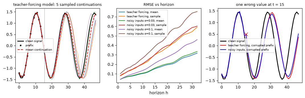
- Errors compound. One step ahead the error is at the noise level, then it grows steadily: every step conditions on values the model produced itself, so small errors in the inferred frequency and phase accumulate. The training loss — one step, true inputs — never measured this.
- Sampled continuations drift about twice as fast as the mean continuation: they carry the model’s own noise forward as if it were signal.
- The distribution survives. Generated from scratch, sequences keep the data’s amplitude statistics over all 48 steps. The drift is away from a particular continuation, not a collapse of the distribution.
Its own errors. Put one wrong value (+0.5) at t = 15 of the prefix and compare the continuation with the clean-prefix continuation:
| model | deviation h = 1 | h = 8 | h = 32 |
|---|---|---|---|
| teacher forcing | 0.266 | 0.461 | 0.960 |
| noisy inputs σ_in = 0.03 | 0.264 | 0.450 | 0.934 |
| noisy inputs σ_in = 0.1 | 0.232 | 0.415 | 0.843 |
None of the models “recovers”: one bad value changes what the window suggests about amplitude and phase, and the continuation follows a different sinusoid. Models trained on noisy inputs are thrown off somewhat less, because they have seen imperfect histories.
The remedy is not free:
- noisy-input training cost one-step likelihood (mean NLL −1.015 vs −1.151 at σ_in = 0.1);
- it made ordinary free-running forecasts worse (0.459 vs 0.317 at h = 32): a model that distrusts its inputs extracts less from a clean prefix.
5. Shared computation, and what “causal” must guarantee
5.1 One network for all conditionals
Teacher forcing makes every conditional’s input known in advance (it is just the data), so all n conditionals can be computed at once. With shared weights, five separate networks with 1–5 inputs collapse into a single network with five outputs. The slides state the condition precisely: one network computes all conditionals, with shared architecture, weights and computation, if output i does not depend on any input x_j with j ≥ i.
The standard implementation:
- feed the sequence [BOS, x₁, …, x_{n−1}] (the data shifted right by one);
- read output i as the distribution of x_i;
- make sure output i only looks at input positions ≤ i.
“Shift target by one step” is the slides’ phrase; the second requirement is what “causal” means.
5.2 Three ways to break it
If output i can see x_i itself, the prediction problem becomes copying. Code 03, part 2 implements three classic bugs on the bracket language (§6.4):
- a Transformer without the causal mask;
- a CNN with ordinary symmetric padding;
- a causal Transformer trained on unshifted targets.
| model | train NLL (bits/char) | test NLL | samples’ NLL under a correct model (“judge”) | distinct samples of 500 |
|---|---|---|---|---|
| Transformer without causal mask | 0.050 | 0.049 | 11.40 | 28 |
| CNN with “same” padding | 0.032 | 0.032 | 6.01 | 500 |
| unshifted targets | 0.001 | 0.001 | 8.03 | 19 |
| (correct causal Transformer, §6.4) | — | 1.841 | 1.84 (real strings) | — |
Losses that look too good to be true are. The leaky models score 50–1800× better than the correct one on training and test data, because the answer is in the input.
At sampling time the answer is not there yet. The model must predict from the past alone, a task it never learned:
- the unmasked and unshifted Transformers degenerate into runs of one character (”[[[[[…”, ”((((((…”);
- the symmetric CNN produces varied strings with brackets closing at random.
Note the unmasked Transformer needed several hundred steps to find the shortcut (at 300 steps its loss was still 2.12 bits), so a short training run would not even have looked suspicious.
The no-peeking test catches all three without any training. Replace x_i, x_{i+1}, … by random tokens and check that the predictions for x_0 … x_i do not move:
- the buggy models change by 0.22–2.0;
- the correct ones by at most 5e−6, which is float rounding inside the convolution.
Run it on every new autoregressive architecture before spending compute.
5.3 Training is parallel; sampling is not
Code 03, part 3 (causal Transformer, 256 strings of 48 characters): one teacher-forced pass computes all 48 conditionals in 23.5 ms, while sampling the same 256 strings takes 638 ms, 27× slower.
Sampling needs one pass per token. It needs even more here, because each pass reprocesses the whole prefix; real systems cache the past keys and values to avoid that. This asymmetry — cheap likelihood, expensive sampling — is the characteristic cost of autoregressive models, and the target of much later work (parallel decoding, MAR’s multi-token steps, speculative decoding).
6. Architectures for autoregression
6.1 Recurrent networks
An RNN unit takes the current input and a hidden state and returns a new hidden state. Unfolded over time, it processes x₁, x₂, … in order; stacking layers makes it deep. Shifting the targets by one turns output i into p(x_{i+1} | x_{≤i}), or equivalently p(x_i | x_{<i}) with the BOS convention. The hidden state is a running summary of the entire past, so memory is in principle unlimited, but it is squeezed into a fixed-size vector and must be computed step by step even during training.
The slides’ example is Char-RNN (Karpathy’s 2015 blog post The Unreasonable Effectiveness of Recurrent Neural Networks). A character-level RNN trained on Shakespeare, Wikipedia markup, LaTeX or C code produces strikingly plausible text, including matching brackets and indentation.
6.2 Causal convolutions
A 1-D convolution along the “time” axis looks at a window of neighbours. With ordinary symmetric padding that window includes the future. A causal convolution pads only on the left, so output i sees inputs ≤ i. Stacking layers grows the receptive field; with dilated convolutions (dilations 1, 2, 4, 8, …) it grows exponentially with depth. That is WaveNet (van den Oord et al. 2016), which generates raw audio sample by sample with dilated causal convolutions. Training is fully parallel, but anything outside the receptive field is invisible.
6.3 Causal attention
Full attention lets every position attend to every position. Causal attention masks the scores above the diagonal so that position i attends only to positions ≤ i. With the shift-by-one convention this is exactly the condition of §5.1. Every position has direct access to the entire past, and training is parallel. image GPT (iGPT, Chen et al. 2020) applies this to pixels: a GPT-style Transformer on images flattened to sequences, predicting x₁ … x_n from x₀ … x_{n−1}. GPT (Radford et al. 2018) does the same with text tokens.
| memory of the past | training | sampling step cost | |
|---|---|---|---|
| RNN | fixed-size summary, unlimited range | sequential | O(1) per token |
| causal CNN | exact, within the receptive field | parallel | O(receptive field) |
| causal attention | exact, everything | parallel | O(length) per token (with a cache) |
6.4 Experiment: a bracket language
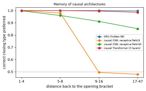
Code 03 trains four correct architectures on strings of 48 characters: letters a–d that follow a successor rule (a→b→c→d→a) with probability 0.8, and nested ( ) [ ] brackets that must close in the right type and order. The letter rule needs a few characters of context. Closing a bracket needs to remember which bracket is open, possibly far back (the median distance is 3, but 10% of the pairs are more than 16 apart).
| model | parameters | test NLL (bits/char) | valid samples (of 500) | closing accuracy, distance 9–16 | distance 17–47 |
|---|---|---|---|---|---|
| GRU | 33,752 | 1.901 | 0.296 | 1.000 | 0.998 |
| causal CNN, receptive field 8 | 25,864 | 2.027 | 0.016 | 0.495 | 0.479 |
| causal CNN, receptive field 64 | 50,632 | 1.911 | 0.326 | 0.912 | 0.852 |
| causal Transformer | 104,328 | 1.841 | 0.808 | 0.996 | 0.986 |
(“Closing accuracy”: with teacher forcing, the model prefers the correct closing bracket over the wrong one.)
-
Receptive field is a hard limit. The receptive-field-8 CNN can see only 7 characters back: for brackets opened further away it guesses (accuracy ≈ 0.5), and almost none of its samples are valid.
-
The GRU remembers perfectly but samples badly. Its teacher-forced bracket memory is perfect (0.998 even at distance 17–47), yet only 30% of its samples are valid. The failure breakdown explains it:
model valid still open at the end wrong type close without open GRU 0.296 0.496 0.148 0.060 causal Transformer 0.808 0.094 0.084 0.014 Most invalid GRU samples are still holding open brackets when the 48 characters run out. The task also requires knowing where you are and starting to close in time. The Transformer has positional embeddings; the GRU must count. Sampling exposes what the teacher-forced loss averages away.
-
Temperature (Char-RNN style). Dividing the logits by T before sampling (GRU):
temperature valid distinct strings (of 500) NLL of samples under the Transformer 0.5 0.840 466 0.93 1.0 0.316 500 2.05 1.5 0.094 500 2.79 T < 1 sharpens every conditional (fewer mistakes, less variety), T > 1 flattens them. Either way it no longer samples the model’s own distribution — the same trade as temperature in flows (Lecture 4 §3.4).
7. The running example: an image as a sequence of pixels
The slides’ running example is AR on MNIST. Treat an image as a sequence of pixels in raster order (left to right, top to bottom).
- At inference, sample pixel 1 from p(x₁), then pixel 2 from p(x₂ | x₁) — the network for this step has one input — and so on. At step n the network has n − 1 inputs, all outputs of previous steps.
- In training (teacher forcing) the n − 1 inputs are ground-truth pixels.
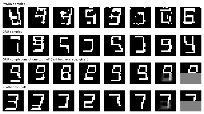
This says nothing about the architecture: it is valid for RNNs, CNNs and Transformers alike. Code 04 runs it on binarized 16×16 glyphs (256 pixels), with four models:
| model | parameters | test bits / pixel | recognizable samples | FID (vs binarized real) |
|---|---|---|---|---|
| independent pixels | 256 | 0.4132 | — | — |
| FVSBN, raster order | 32,896 | 0.1604 | 0.718 | 117.6 |
| FVSBN, a random fixed order | 32,896 | 0.1548 | 0.680 | 111.6 |
| local MLP, 12-pixel causal neighbourhood (shared) | 22,401 | 0.1282 | 0.741 | 132.4 |
| GRU over the raster sequence (shared) | 37,825 | 0.1313 | 0.792 | 88.8 |
| (held-out binarized real images) | — | — | 0.974 | 4.3 |
The models:
- FVSBN (fully visible sigmoid belief net) gives every pixel its own logistic regression on all previous pixels: no weight sharing. It is the starting point of Bengio & Bengio (1999) and of Lecture 6.
- Local MLP: one shared MLP sees two rows above and two pixels to the left.
- GRU: one shared recurrent network reads the whole raster sequence.
- Conditioning is where the information is. Every autoregressive model needs well under half the bits of the independent-pixel model.
- Shared weights generalize. The local MLP, with fewer parameters than FVSBN, beats it clearly. A stroke looks the same everywhere, so one shared rule “continue the stroke” serves all 256 positions, while FVSBN learns it position by position.
- The random order surprised me. For FVSBN it is slightly better than raster order. A plausible reason: in a random order a late pixel already knows neighbours on all sides, and a logistic regression can interpolate, while raster order only ever shows the upper-left half. Both are exact chain rules; which one suits a given family is an empirical question (§2.2).
- Best likelihood ≠ best samples. The local MLP has the best likelihood but the worst FID. It sees only two rows up, so every stroke is locally plausible while the digit as a whole may not hang together. Likelihood averages 256 mostly local predictions; sample quality depends on global coherence. The GRU, with its running memory of everything above, gives the best samples.
- Errors in samples compound. A fifth to a third of the samples are not recognizable: one wrong pixel early in a stroke is never corrected (§4.4, in two dimensions).
- No copying. Hardly any sample reproduces a training image exactly — fewer than held-out real images do, since binarization makes 7.4% of real glyphs coincide with a training glyph.
Completing the bottom half. Give the GRU the top 8 rows of 100 test glyphs, and sample the bottom 8 rows 20 times each. In GlyphWorld the top half is often genuinely ambiguous: when the middle bar falls below row 8, 2/3/7 share a top half, and so do 0/8/9.
Because we know the generating process, the set of consistent digits is computable exactly: re-render each test glyph as every digit with the same style, and keep the digits whose binarized top half is identical. The top halves fit 2.01 digits on average, and 69% fit two or more.
| completion | recognizable | consistent with the top half (among recognizable) | gray pixels per image |
|---|---|---|---|
| each of the 20 samples | 0.797 | 0.766 | 0.0 |
| their average (≈ the conditional mean, i.e. regression) | 0.700 | 0.971 | 32.1 |
- Sampling represents the ambiguity. Each sampled completion is a crisp binary glyph, and the completions of one top half spread over several digits. In the figure, one top half finishes as 3, 2 and 7. This is what Lecture 1 asked of a generative model: represent the one-to-many conditional distribution, then sample from it.
- Not every completion respects the top half. About a quarter of the recognizable ones end as a digit the top half rules out, so the completions spread over 3.1 digits per top half where only 2.0 are possible. A stroke continued wrongly near the middle is never undone.
- The average is Lecture 1’s ghost. It has 32 gray pixels per image where the completions disagree. The classifier often still names a plausible digit, but it is not a glyph.
8. The big picture
8.1 The slides’ takeaways
- Joint distribution ⇒ product of conditionals.
- Inductive bias: shared architecture, shared weights, induced order.
- Inference: autoregressive. Training: teacher forcing.
- Can be done by RNNs, CNNs and Transformers.
8.2 Autoregression in the five-component framework
| Component | Autoregressive model |
|---|---|
| formulation | chain rule over an order and a partition of x; a dependency graph |
| representation | one shared causal network (RNN / causal CNN / causal Transformer) outputting a distribution per position (softmax, or a density) |
| objective | exact log-likelihood = sum of per-position cross-entropies |
| optimization | SGD with teacher forcing; all positions in parallel |
| inference | sequential sampling, n steps (temperature optional); exact likelihood of any x in one pass |
8.3 Strengths and costs, compared with Lectures 3–4
| VAE | flow | autoregressive | |
|---|---|---|---|
| likelihood | lower bound | exact | exact |
| architecture constraint | none | invertible, cheap log-det | causal (“no peeking”) |
| latent space | yes (compressed) | yes (full-dimensional) | none |
| sampling | one pass | one pass | n sequential passes |
| typical failure | blur | bridges, speckle | compounding errors, slow sampling |
The causal constraint is far milder than invertibility, which is why autoregressive models scaled to the largest generative models in existence (language models).
Their costs:
- sequential sampling;
- a fixed order and partition to choose;
- exposure bias — the model never sees its own errors in training.
Lectures 6–8 work on each: better architectures (NADE, PixelCNN), better units (tokens instead of pixels, Lecture 7), and better orders and partitions (masked / random-order AR with continuous tokens, Lecture 8).
9. Summary
- Dependence is the whole problem. Independent variables (or independent latents) are easy but too strict for high-dimensional data, unless the latent is exactly right. In our 7-bit world a 10-class latent is exact; one class costs the full total correlation, 1.17 bits.
- The chain rule makes no approximation, in any order and any partition. What x_i means (pixels, VQ tokens, noise levels) is a design choice.
- Approximation enters through inductive bias: the family of each conditional, shared architecture and weights, and the dependency graph.
- Logistic conditionals cost 0.2 bits in every order.
- A chain graph costs 0.54–1.11 bits depending on the order.
- Predicting blocks of variables independently costs their within-block dependence.
- One conditional is one network output: a softmax (a classifier) for discrete variables, or a density for continuous ones.
- Inference is autoregressive; training is teacher-forced. Backpropagating through the inference graph is infeasible. Teacher forcing is parallel and stable, but the model never sees its own errors: free-running errors compound, and remedies such as noisy inputs trade one problem for another.
- Shared computation requires that output i not depend on inputs at j ≥ i, with the targets shifted by one. Violations make the loss look wonderful and the samples useless; a no-peeking test catches them before training.
- RNNs, causal CNNs and causal attention differ in memory (summary / receptive field / everything) and in parallelism. Teacher-forced metrics can hide sampling failures (the GRU that remembers brackets but cannot count).
- Pixels in raster order work. Shared weights beat per-pixel weights, likelihood and sample quality can disagree, and sampled completions represent the one-to-many conditional that regression averages into a ghost.
10. Common pitfalls
- “Autoregressive means recurrent.” Autoregression is a formulation (the chain rule) plus sequential inference. It can be implemented by RNNs, CNNs, Transformers, or lookup tables (§4.1, §6).
- “Autoregressive models need a natural order (time).” Any order and any partition are valid. Time order is an inductive bias, and other orders can be easier for a given family (§2.3, §7).
- “The chain rule is an approximation.” It is an identity. The approximations are the conditional families, shared weights and restricted dependency graphs.
- “Training is autoregressive too.” Training uses teacher forcing: ground-truth inputs, all positions in parallel (§4.3).
- “Low teacher-forced loss means good samples.” Free-running errors compound (§4.4); a model can be excellent per step and still fail globally (§6.4: the GRU; §7: the local MLP).
- “My model’s loss is tiny, great!” Check for peeking: a missing causal mask, symmetric padding or unshifted targets all produce near-zero losses (§5.2).
- “Sampling is as cheap as evaluating the likelihood.” Likelihood takes one parallel pass; sampling takes one pass per position (§5.3).
- “Lower temperature gives better samples.” It gives sharper but less diverse samples from a different distribution (§6.4).
- “Exact likelihood means the model knows the structure.” Likelihood can be dominated by local predictions while global structure fails (§7).
11. Exercises
Exercise 1 (the chain rule). (a) Derive p(A, B, C) = p(A)p(B | A)p(C | A, B) from the definition of conditional probability. (b) For n binary variables, how many free parameters does a full table of conditionals have in any order? Compare with the full joint table. (c) Why does the answer in (b) not depend on the order?
Answer
(a) p(C | A, B) = p(A, B, C)/p(A, B) and p(B | A) = p(A, B)/p(A). Multiply: p(A) · p(A,B)/p(A) · p(A,B,C)/p(A,B) = p(A,B,C).
(b) The i-th conditional needs one number per configuration of its i − 1 parents: Σ_{i=1}^n 2^{i−1} = 2^n − 1. That is exactly the size of the joint table minus 1 (normalization).
(c) Both count the same object: an arbitrary distribution over 2^n outcomes. The chain rule is a re-parameterization, not a restriction. Restrictions (logistic conditionals, fewer parents) are what make orders differ.
Exercise 2 (independent prediction of a block). Show that if a model predicts the variables of a block B independently given the past P, using the exact marginal conditionals p(x_j | P), its expected excess log-loss over the exact joint conditional is Σ_{j∈B} H(x_j | P) − H(x_B | P) ≥ 0, the conditional total correlation. When is it zero?
Answer
The model’s log-loss for the block is E[−Σ_j log p(x_j | P)] = Σ_j H(x_j | P). The exact conditional’s is H(x_B | P). Their difference is the KL between p(x_B | P) and Π_j p(x_j | P), averaged over P, hence ≥ 0. It is zero iff the variables of the block are conditionally independent given the past. In code 01 the cost grows from 0.11 bits (pairs) to 1.17 bits (all seven at once).
Exercise 3 (a logistic conditional with one parent). Show that any conditional distribution of a binary x given one binary parent y can be written as σ(w·y + b). Why does that stop being true with two parents?
Answer
With one binary parent there are two numbers to match, p(x=1 | y=0) and p(x=1 | y=1). Choose b = logit p(x=1|y=0) and w = logit p(x=1|y=1) − b.
With two parents there are four probabilities but σ(w₁y₁ + w₂y₂ + b) has three parameters. The logit must be additive in the parents, so an interaction (e.g. XOR-like dependence) cannot be represented without an extra feature y₁y₂. This is why, in code 01, the logistic family is exact for early conditionals and loses bits late.
Exercise 4 (teacher forcing as maximum likelihood). Show that the teacher-forced loss Σ_i −log p_θ(x_i | x_{<i}), with x from the data, is exactly the negative log-likelihood −log p_θ(x). Why is that not true of a loss computed on the model’s own rollouts?
Answer
By the chain rule, log p_θ(x) = Σ_i log p_θ(x_i | x_{<i}) evaluated at the data x. So teacher forcing is maximum likelihood, nothing more. A rollout replaces x_{<i} by samples x̂_{<i}. The quantity Σ_i −log p_θ(x_i | x̂_{<i}) is not the likelihood of anything; it mixes data targets with model histories. It measures something closer to robustness to the model’s own errors, which is why rollout-based training needs its own justification (and its own gradient estimators for the sampling steps).
Exercise 5 (causal convolution). A stack of L causal convolutions with kernel size 2 and dilations 1, 2, 4, …, 2^{L−1}: (a) show that the receptive field is 2^L; (b) how many layers does a sequence of length 16,000 (one second of 16 kHz audio) need? (c) Why does left-padding by the dilation keep the convolution causal?
Answer
(a) A layer with dilation d sees positions t − d and t, adding d to the receptive field. Starting from 1, the total is 1 + Σ_{l<L} 2^l = 2^L.
(b) 2^14 = 16,384 ≥ 16,000, so 14 layers. WaveNet repeats such stacks several times.
(c) Output t combines inputs t − d and t; padding d zeros on the left makes position 0’s “t − d” a zero instead of shifting the window right. No future input ever enters.
Exercise 6 (the causal mask). Write the attention scores for a sequence of length 4 with the causal mask applied. Show that with inputs [BOS, x₁, x₂, x₃] and the mask, output 2 is a function of BOS, x₁ only. What exactly goes wrong if the targets are not shifted?
Answer
The mask sets s_{ij} = −∞ for j > i, so row i of the softmax only weighs columns 0..i.
Output 2 (0-indexed, i.e. the third output) attends to inputs 0, 1, 2 = BOS, x₁, x₂, and is trained to predict x₃. Equivalently, output i predicts x_{i+1} from BOS, x₁..x_i. Renaming positions gives p(x_i | x_{<i}).
Without the shift, the input at position i is x_i, and the causal mask still allows position i to attend to itself. The model learns to copy (code 03: loss 0.001 bits), and at inference the token to copy does not exist yet.
Exercise 7 (sampling cost). A causal Transformer with L layers and width d generates n tokens. (a) Estimate the cost of one teacher-forced pass and of naive sampling (re-running the prefix every step). (b) How does caching keys and values change the sampling cost?
Answer
(a) One pass costs about L(n·d² + n²·d): projections plus attention. Naive sampling runs passes on prefixes of length 1..n, so roughly L(n²d²/2 + n³d/3) — a factor of order n more.
(b) With a cache, step t only computes the new token’s projections (L·d²) and its attention over t cached keys (L·t·d), so the total is about L(n d² + n² d/2). That is the same order as one teacher-forced pass, but executed as n sequential steps that cannot be parallelized.
Exercise 8 (temperature). Sampling at temperature T samples from q_T(x_i | x_{<i}) ∝ p(x_i | x_{<i})^{1/T} at each step. Is the resulting distribution over whole sequences proportional to p(x)^{1/T}? Why or why not?
Answer
Not in general. Each step renormalizes, so q_T(x) = Π_i p(x_i | x_{<i})^{1/T} / Z_i(x_{<i}), with a normalizer Z_i that depends on the history. p(x)^{1/T} would need a single global normalizer. The two agree only if all Z_i are equal, for example when every conditional has the same entropy profile. Per-step temperature is a different, history-dependent tilt.
Exercise 9 (hands-on).
(a) In 03_causal_architectures.py, give the GRU the position t/48 as an extra input. Does the share of “still open at the end” samples drop?
(b) In 04_pixel_ar.py, train FVSBN in a “snake” order (left to right, then right to left on the next row). Is it closer to raster or to random?
(c) In 02_teacher_forcing.py, implement scheduled sampling: with probability ρ, replace an input by the model’s own sampled prediction (computed without gradient). Compare ρ = 0.25 with the noisy-input models.
Answer (sketch)
(a) Expect a large drop if the diagnosis in §6.4 is right: with the position known, the GRU can learn “close everything when as many positions remain as brackets are open”. Your run decides.
(b) The snake order keeps a left or right neighbour and the upper row available, much like raster order, so expect a likelihood near raster. The random order’s advantage (neighbours on all sides) does not appear.
(c) Scheduled sampling shows the model its own errors, not artificial Gaussian noise, so it can be more targeted. Expect a trade-off similar to the noisy inputs: better robustness to injected errors, some cost in one-step likelihood.
12. Further reading
The slides’ main references
- Y. Bengio & S. Bengio, Modeling High-Dimensional Discrete Data with Multi-Layer Neural Networks, NeurIPS 1999 (Lecture 6).
- A. van den Oord, N. Kalchbrenner, K. Kavukcuoglu, Pixel Recurrent Neural Networks, ICML 2016 (Lecture 6).
- A. Radford, K. Narasimhan, T. Salimans, I. Sutskever, Improving Language Understanding by Generative Pre-Training, 2018 (GPT).
Also cited on the slides
- D. P. Kingma & M. Welling, Auto-Encoding Variational Bayes, ICLR 2014 (the VAE MNIST samples).
- T. Li, Y. Tian, H. Li, M. Deng, K. He, Autoregressive Image Generation without Vector Quantization, 2024 (MAR, Lecture 8).
- T. Hua et al., Self-supervision through Random Segments with Autoregressive Coding (RandSAC) (cited on the slides as ICLR 2022).
- A. Karpathy, The Unreasonable Effectiveness of Recurrent Neural Networks, blog post, 2015.
- A. van den Oord et al., WaveNet: A Generative Model for Raw Audio, 2016.
- M. Chen et al., Generative Pretraining from Pixels (iGPT), ICML 2020.
Background
- S. Bengio, O. Vinyals, N. Jaitly, N. Shazeer, Scheduled Sampling for Sequence Prediction with Recurrent Neural Networks, NeurIPS 2015.
- A. Vaswani et al., Attention Is All You Need, NeurIPS 2017.
- T. Salimans et al., PixelCNN++, ICLR 2017: discretized logistic mixtures for pixel conditionals.
Related notes in this course
- Lecture 1 §2 (one-to-many and ghosts), §6.4 (the smallest autoregressive model and factorization order).
- Lecture 3 §7 (VQ-VAE tokens, the units of Lecture 7).
- Prerequisite P2 §4 (attention, causal masks and the shared computation of teacher forcing).
13. Next lecture
Lecture 6: Classic autoregressive models — from NADE to PixelCNN and IAF (reading session · 09/24; Problem Set 2).
This lecture’s FVSBN gave every pixel its own logistic regression. The three papers of Lecture 6 improve it in three directions:
- Bengio & Bengio (1999) replace per-variable tables with neural networks that share hidden units across conditionals — the ancestor of NADE and MADE.
- PixelRNN / PixelCNN (2016) bring deep 2-D architectures to raster-order pixels: row LSTMs, diagonal BiLSTMs, and masked convolutions (type A and B) whose “blind spot” we will find with gradients.
- Inverse autoregressive flows (2016) turn the autoregressive structure into a flow with a triangular Jacobian, closing the loop with Lecture 4. MAF evaluates densities fast and samples slowly; IAF does the opposite.
Problem Set 2 asks for the NLL = cross-entropy proof and a masked-convolution PixelCNN; we will do both on binarized glyphs.