Lecture 12 · Energy-Based Models, Score Matching and Diffusion Models

Maps to: MIT 6.S978 Deep Generative Models (Fall 2024), Lecture · Thu 10/17/2024 · Energy-based Models, Score Matching, Diffusion Models (slides: lec5_diffusion.pdf, Kaiming He). Problem Set 4 (released 10/22):

• DDPM on MNIST: schedule, forward process, sampling;
• ablations of the number of timesteps and of the number of sampling steps;
• continuous time: marginals and analytic scores of a two-Gaussian mixture under the VP-SDE.

Basis: The order and content follow the slides — diffusion models (forward process, reverse process, training objective, noise-conditional network), then energy-based models and score matching. Their derivations are written out in full: the closed-form forward process, the Gaussian posterior, KL → L2 on the noise, the variational bound, denoising score matching, Langevin dynamics. All of Problem Set 4 is done: the DDPM on glyphs (in a latent space, §5.3), its ablations, and the VP-SDE derivations as worked solutions (§8). Experiments were designed for these notes and run on a CPU. Several outcomes refined or contradicted my expectations and are reported as they came out:

• training with the ELBO’s weights failed through gradient variance, and worked with importance sampling;
• T = 500 beat T = 1000 with the problem set’s schedule;
• a pixel-space MLP denoiser was too weak, which is why the glyph DDPM runs in Lecture 8’s latent space.

Code: code/lecture12/ — 7 scripts + the shared module diffusion.py. They run in 1–125 s. Reading time: 5 hours including running the code.

0. How to read this lecture

0.1 Where we are

The slides open with a timeline: diffusion models were proposed in 2015 (Sohl-Dickstein et al.), largely ignored for five years, and then — after DDPM (Ho et al. 2020) and score-based models (Song & Ermon 2019) — boomed. Today they and their relatives (flow matching, Lectures 16–17) power most image, video and audio generators.

We now have every ingredient to see why:

• Lecture 3: the VAE’s ELBO — and diffusion’s objective is an ELBO;
• Lecture 5: “divide and conquer” by a chain of simple conditionals — and diffusion chains many Gaussian conditionals;
• Lecture 8: a one-page preview of noising and denoising;
• Lecture 11: samples moving along a score difference.

This lecture builds diffusion models properly. It then shows that they are a form of score matching, an old idea for training energy-based models.

0.2 Learning goals

1. Derive the forward process in closed form, explain the role of the schedule, and check that its end is “all noise” (§2).
2. Explain why the reverse conditional q(x_{t−1} | x_t) is unknown but q(x_{t−1} | x_t, x_0) is a known Gaussian; derive its mean and variance; turn the KL into an L2 loss on the noise (§3).
3. Derive the training objective from the variational bound, and explain “set the weights as 1 (critical)” (§4).
4. Describe the noise-conditional network and the training and sampling algorithms; implement Problem Set 4’s DDPM and its ablations (§5).
5. Define energy-based models, score functions, score matching (explicit, sliced, denoising) and Langevin dynamics, and connect them to diffusion (§6–7).
6. Solve Problem Set 4’s continuous-time problem: VP-SDE marginals, scores, the reverse SDE and the probability-flow ODE (§8).

0.3 Map

1. Diffusion in a nutshell

The slides compress the idea into two pictures:

• Forward process: add noise. Data → slightly noisy → … → pure noise, by many small, fixed steps. Nothing is learned.
• Reverse process: denoise. Pure noise → … → data. Each small step back is learned.

What is noise? The slides answer with an equivalence: adding Gaussian noise to a sample ⇔ sampling from the convolution of its density with a Gaussian. If x ~ p, then x + σε ~ p * N(0, σ²). Noise blurs a distribution: modes widen, merge, and eventually the distribution becomes a single broad Gaussian — easy to sample.

Code 01 (part 1) checks this on a 1-D mixture 0.3·N(−2, 0.3²) + 0.7·N(1.5, 0.5²). The histograms of x + σε match p * N(0, σ²) to histogram precision. The two modes, 3.5 apart, merge between σ = 1 and σ = 2. But the variance keeps growing (2.8 → 18.8 at σ = 4). DDPM therefore also shrinks the data at every step, so that the end point is a fixed N(0, I).

Divide and conquer. Generating data from noise in one step is hard: one map from N(0, I) to the data distribution. Generating one slightly less noisy version of a noisy sample is easy, as §3 shows. Diffusion splits the hard problem into T easy ones — the chain rule of Lecture 5, applied along a noise axis instead of across pixels.

2. The forward process

2.1 The step and its coefficients

• Variance preserving. If $\operatorname{Var}(x_{t-1}) = 1$, then $\operatorname{Var}(x_t) = \alpha_t + (1 - \alpha_t) = 1$: the coefficients are chosen so the scale never explodes.
• The noise is i.i.d. It is independent across dimensions (the identity covariance), with the same dimension as the data.
• The schedule $\beta_1, \dots, \beta_T$ — “key to diffusion models’ success”, in the slides’ words — fixes how fast the data is destroyed.

Problem Set 4, 1(a) uses the linear schedule $\beta_t = \beta_{\min} + \frac{t - 1}{T - 1}(\beta_{\max} - \beta_{\min})$ with β from 1e-4 to 0.02 and T = 1000, and $\bar\alpha_t = \prod_{s \le t} \alpha_s$ (ddpm_schedules).

2.2 Sampling without simulation

Claim. $q(x_t \mid x_0) = \mathcal N(\sqrt{\bar\alpha_t}\, x_0,\ (1 - \bar\alpha_t) I)$.

Derivation (Problem Set 4, 1(b)). Unroll two steps:

The two noise terms are independent Gaussians, so their sum is Gaussian with variance $\alpha_t(1 - \alpha_{t-1}) + (1 - \alpha_t) = 1 - \alpha_t \alpha_{t-1}$. Hence $x_t = \sqrt{\alpha_t\alpha_{t-1}}\, x_{t-2} + \sqrt{1 - \alpha_t\alpha_{t-1}}\, \bar\varepsilon$. By induction,

Training never simulates the chain: draw t, draw ε, compute $x_t$ in one line (q_sample).

Code 01 (part 2) iterates the chain for one glyph with 4000 noise draws. After t steps every pixel has mean $\sqrt{\bar\alpha_t} x_0$ and variance $1 - \bar\alpha_t$ to Monte-Carlo precision:

(The standard error of a mean over 4000 chains is ≈ 0.015; the table shows the worst of 256 pixels.)

2.3 The schedule, and whether x_T is pure noise

How much signal survives is best read through the log signal-to-noise ratio, $\log(\bar\alpha_t / (1 - \bar\alpha_t))$:

The linear schedule reaches “as much noise as signal” by t ≈ 250 and spends its last quarter below log-SNR −5.7, at almost pure noise. The cosine schedule (Nichol & Dhariwal 2021) keeps more signal in the middle.

Is the end “all noise”? The sampler starts from N(0, I), so we want $q(x_T \mid x_0) \approx \mathcal N(0, I)$. For glyph pixels in [−1, 1]:

With the problem set’s β range, T = 500 leaves √ᾱ_T ≈ 8% of the image in x_T. §5.4 measures whether that matters (it barely did).

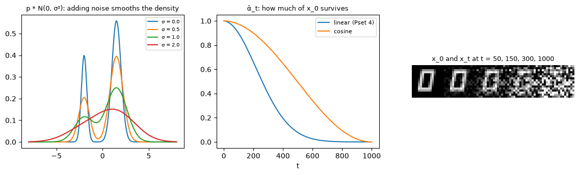
The slides’ summary of the forward process: pre-defined conditional distributions; Gaussian with controllable mean and std; divide and conquer.

3. The reverse process

3.1 The target is unknown

We want to run the chain backward: $q(x_{t-1} \mid x_t)$. By Bayes, it is $q(x_t \mid x_{t-1})\, q(x_{t-1}) / q(x_t)$, and $q(x_{t-1})$ is the data distribution blurred to level t-1. The slides’ picture: several different $x_{t-1}$ could have produced the same $x_t$, and how likely each one is depends on the data.

So the reverse conditional is our target, but unknown. We represent it by a network, $p_\theta(x_{t-1} \mid x_t)$, a Gaussian whose mean (and possibly variance) the network outputs.

3.2 Conditioned on x_0, it is a known Gaussian

$q(x_{t-1} \mid x_t, x_0)$ is not our target but known. Both factors in $q(x_{t-1} \mid x_t, x_0) \propto q(x_t \mid x_{t-1})\, q(x_{t-1} \mid x_0)$ are Gaussians in $x_{t-1}$, so their product is too.

• Precision (inverse variance): $$\frac{\alpha_t}{\beta_t} + \frac{1}{1 - \bar\alpha_{t-1}} = \frac{\alpha_t(1 - \bar\alpha_{t-1}) + \beta_t}{\beta_t (1 - \bar\alpha_{t-1})} = \frac{1 - \bar\alpha_t}{\beta_t(1 - \bar\alpha_{t-1})} .$$
• Variance and mean: $$\tilde\beta_t = \frac{1 - \bar\alpha_{t-1}}{1 - \bar\alpha_t}\,\beta_t, \qquad \tilde\mu_t(x_t, x_0) = \frac{\sqrt{\bar\alpha_{t-1}}\,\beta_t}{1 - \bar\alpha_t}\, x_0 + \frac{\sqrt{\alpha_t}\,(1 - \bar\alpha_{t-1})}{1 - \bar\alpha_t}\, x_t .$$

The mean is a linear combination of $x_0$ and $x_t$, and the variance depends only on the schedule: “the outcome of the dependency graph, some linear combinations”. Code 02 (part 1) confirms all three numbers by simulation. It fixes x_0 = 1.3, draws 400,000 pairs $(x_{t-1}, x_t)$ and regresses one on the other:

Written with the noise. Substitute $x_0 = (x_t - \sqrt{1 - \bar\alpha_t}\,\varepsilon)/\sqrt{\bar\alpha_t}$ and simplify (the coefficients of $x_t$ combine to $1/\sqrt{\alpha_t}$):

The “noise” ε is the only unknown in the mean.

3.3 Why many small steps

How wrong is it to model $q(x_{t-1} \mid x_t)$ — the unknown one — as a Gaussian? Code 02 (part 2) computes it exactly for the 1-D mixture (Bayes on a fine grid). It measures its KL to the best Gaussian fit, averaged over 100 values of x_t:

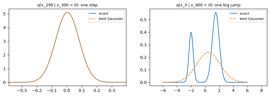
• One small step back is Gaussian to 10⁻⁷ nats or better, so a Gaussian $p_\theta$ loses essentially nothing and only its mean must be learned. That is the justification for many small steps.
• Big jumps that land near the data are bimodal. A noisy $x_t$ is compatible with both modes, and a Gaussian step must average them (Lecture 1’s ghost).
• A big jump between two noise-dominated levels (900 → 500) is still nearly Gaussian. The difficulty lives at the low-noise end, where the data’s structure appears.

3.4 From KL to an L2 loss on the noise

Represent $p_\theta(x_{t-1} \mid x_t) = \mathcal N(\mu_\theta(x_t, t), \sigma_t^2 I)$ with a preset variance $\sigma_t^2$ ($\beta_t$ or $\tilde\beta_t$; DDPM found both work). The KL between two Gaussians with the same variance is an L2 distance between the means — Problem Set 1’s result, which the slides recall:

Give $\mu_\theta$ the same form as $\tilde\mu_t$, with a network $\varepsilon_\theta$ in place of the unknown noise: $\mu_\theta = \frac{1}{\sqrt{\alpha_t}}(x_t - \frac{\beta_t}{\sqrt{1 - \bar\alpha_t}}\varepsilon_\theta(x_t, t))$. Then

“Learn → preset → ‘noise’ → estimate noise”: a network to predict noise; input: noisy image. Code 02 (part 3) checks the identity to six digits and prints the weights: with $\sigma_t^2 = \tilde\beta_t$, λ_t ranges from 0.005 to 0.6 (a factor of 120), largest at the smallest t.

4. The training objective

4.1 A variational bound

Treat $x_{1:T}$ as latent variables of a hierarchical VAE whose “encoder” is the fixed forward process $q(x_{1:T} \mid x_0)$ and whose “decoder” is the reverse chain $p_\theta(x_{0:T}) = p(x_T)\prod_t p_\theta(x_{t-1} \mid x_t)$. Exactly as for the ELBO of Lecture 3 (it is the ELBO if T = 1):

The slides read the three terms one by one:

• $L_T$ has no parameters, unlike the VAE’s $q_\phi$: it compares a fixed Gaussian with the constant prior. §2.3 measured it: 0.004 nats per image for Problem Set 4’s schedule.
• $L_{t-1}$ is the KL of §3.4, an L2 loss on the noise, weighted by λ_t.
• $L_0$ is a reconstruction loss, as in the VAE.

4.2 “Set as 1 (critical)”

Averaging over t uniformly, the bound is $\mathbb E_{t, x_0, \varepsilon}[T \lambda_t \|\varepsilon - \varepsilon_\theta\|^2] + \dots$. Ho et al. (2020) dropped the weights:

The slides call this the critical step: a weighted sum of ELBO terms becomes one plain regression, which trains stably and gives the best samples. Salimans & Ho (2022) study the choice of weighting in depth.

4.3 Experiment: three objectives in 2-D

Code 03 trains $\varepsilon_\theta$ (an MLP) on 8 Gaussians of std 0.1 on a ring with three objectives (two seeds). It reports sample quality and the bound itself in nats per point; the true $-\mathbb E \log p_{\text{data}}$ is 0.323.

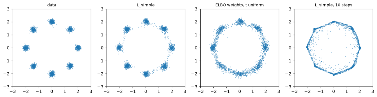
I expected the ELBO weights to give the best bound and worse samples. Instead, with uniform t they gave the worst bound and the worst samples. λ_t varies by 120×, so a few small-t terms dominate every minibatch gradient. Drawing t with probability ∝ λ_t optimizes the same objective with low variance, and it gave the best bound — with samples at least as good as L_simple’s. In 2-D, the weights matter through the variance of the gradient.

4.4 Experiment: the weights on glyphs

On glyphs (code 04, part 3; DDPM on Lecture 8’s latents, §5.3), the importance-sampled ELBO objective again gives the better bound, but now clearly worse samples:

This is Ho et al.’s finding in miniature. The ELBO’s weights concentrate on the smallest noise levels, where the network learns to remove the last traces of noise: fine detail that matters for likelihood but barely for how the glyph looks. Weights of 1 spend relatively more effort at the noisy levels, which decide each glyph’s overall shape. Likelihood and sample quality ask for different weightings — the trade-off behind “set as 1 (critical)”.

5. The noise-conditional network, the algorithms, and Problem Set 4

5.1 One network for all levels

Diffusion decomposes one hard distribution into T simpler conditionals, which would need T networks. Instead, one network conditioned on the noise level fits all of them: the Noise Conditional Score Network (NCSN) of Song & Ermon (2019), “things made work”.

• Inputs: the noisy image $x_t$ and the level t, as an embedding added inside the network.
• Output: the predicted noise $\varepsilon_\theta$, the same size as the input (a U-Net or a ViT). Predicting the noise from a noisy image, the network “behaves like a denoising autoencoder”.

5.2 The algorithms, annotated

Training (repeat until converged)                        Sampling
  x_0 ~ data                                               x_T ~ N(0, I)
  t ~ Uniform{1, …, T}                                     for t = T, …, 1:
  ε ~ N(0, I)                                                  z ~ N(0, I) if t > 1 else 0
  gradient step on ‖ε − ε_θ(√ᾱ_t x_0 + √(1−ᾱ_t) ε, t)‖²       x_{t−1} = (x_t − (1−α_t)/√(1−ᾱ_t) · ε_θ(x_t, t)) / √α_t + σ_t z
                                                           return x_0

The sampling line is “estimated μ, then sample from the estimated distribution” — Problem Set 4, 1(c). ddpm_sample implements it, and also uses it with fewer steps: jumps between levels of an evenly spaced subsequence use the same posterior formula with α = ᾱ_t/ᾱ_s. In the slides’ words: “turns out to be extremely simple”, and being simple and effective moves the needle.

The slides’ examples (Ho et al. 2020):

• unconditional CIFAR-10 samples emerging from noise;
• “shared intermediate latents”: start several reverse chains from the same intermediate $x_t$. From a very noisy $x_t$ the results differ entirely; from a mildly noisy one they share coarse structure. The reverse process decides coarse content first and detail last.

5.3 Problem Set 4, problem 1 on glyphs: pixels vs latents

Problem Set 4 trains a pixel-space DDPM on MNIST with a U-Net on a GPU. On our CPU a convolutional U-Net would need minutes per 1000-step sampling run (3×3 convolutions at 16×16 cost ~9 ms per layer here). Code 04 therefore uses an MLP denoiser, which is fast, and compares two spaces:

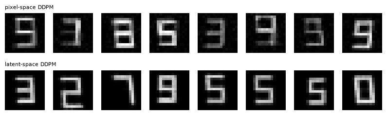
On pixels, the MLP leaves blotchy, half-formed strokes. On the tokenizer’s 64 smooth numbers the same algorithm produces clean glyphs. The pixel space is 4× larger and an MLP has no notion of locality — the reason pixel diffusion uses U-Nets, and the reason latent diffusion (Lecture 13) moved the whole process into an autoencoder’s latent space. The rest of the glyph experiments use the latent DDPM.

5.4 Problem Set 4, problem 2: steps and timesteps

An inference schedule with fewer steps (2.2; code 04, part 2). The network is trained once on all 1000 levels; only the sampler changes:

100 steps lose almost nothing, which is a 10× speed-up for free; 50 lose some; 20 clearly degrade.

In 2-D (code 03, part 2), going from 1000 to 50 steps made samples slightly tighter (spread 0.156 → 0.137). Each big jump injects the posterior variance of a single step, too little — the effect Lecture 8 §2.4 saw. Below ~20 steps they spread out and leave the modes, as §3.3 predicts for big Gaussian jumps.

The number of training timesteps (2.1; code 05). With the problem set’s schedule (β from 1e-4 to 0.02 whatever T is):

I expected T = 500 to be the worst, since its chain does not reach pure noise. It was the best. Starting from N(0, I) instead of the true $q(x_T)$ costs only 0.2 nats. And with β_max = 0.04, the same T = 500 ends in pure noise and performs exactly like T = 1000.

So the number of steps was not what mattered; the range of noise levels was. The T = 500 / 0.02 schedule never goes below log-SNR ≈ −5, while the T = 1000 schedule spends its last quarter at almost pure noise (§2.3). T = 2000 spreads the same 6000 training steps over twice as many levels and costs twice the sampling time. Lecture 13 returns to the lesson: choose the noise schedule and its endpoint carefully — more than the step count.

6. Energy-based models

The slides’ second part: diffusion models are closely related to score matching, and score matching is one solution to training energy-based models (EBMs). Many concepts co-evolved: annealed importance sampling (Neal 1998), denoising score matching (Vincent 2011), the noise-conditional score network (Song & Ermon 2019).

Energy. Define a scalar function E(x). At inference time, find the x that minimizes the energy. In this general sense EBMs can be probabilistic or not, generative or discriminative (LeCun et al.’s tutorial, 2006: inference is energy minimization).

A probability from an energy.

Any energy network defines a density, but Z is an intractable integral in high dimensions. Maximum likelihood needs $\nabla_\theta \log Z$, which requires sampling from the model itself: the classic difficulty of EBMs.

The score function sidesteps Z:

The score needs no normalizing constant. EBMs are therefore “non-normalized probabilistic models”, and a model of the score is enough both to train (§7) and to sample (Langevin, §7.3).

7. Score matching and Langevin dynamics

7.1 Score matching

Instead of parameterizing p, parameterize the score, $s_\theta(x) \approx \nabla_x \log p_{\text{data}}(x)$, and minimize the Fisher divergence:

The data score is unknown. Hyvärinen (2005) expands the square and integrates the cross term by parts (assuming p vanishes at infinity):

So the objective equals, up to a constant,

computable from samples alone. The trace costs one backward pass per dimension. Sliced score matching (Song et al. 2019) projects onto random directions v, $\mathbb E[v^\top \nabla_x(v^\top s_\theta) + \tfrac12 (v^\top s_\theta)^2]$, at the cost of one pass.

7.2 Denoising score matching

Vincent (2011) noises the data, $\tilde x = x + \sigma\varepsilon$, and proves

Proof sketch. Both sides share $\mathbb E\|s_\theta\|^2$. For the cross term,

The remaining terms do not depend on θ.

The conditional score is known: $\nabla_{\tilde x} \log q(\tilde x \mid x) = -(\tilde x - x)/\sigma^2 = -\varepsilon/\sigma$. So the network learns to predict the (negative, scaled) noise, and its optimum is the score of the noised data. For the diffusion process, $\nabla \log q(x_t \mid x_0) = -\varepsilon/\sqrt{1 - \bar\alpha_t}$, so

DDPM’s noise predictor is a scaled score model.

7.3 Langevin dynamics

Given a score, sample p by iterating

This needs the score, not p. As η → 0 with many steps, the stationary distribution is p. In the slides’ reading: a “learning rate” times a gradient plus a perturbation — gradient descent in the energy landscape, with noise.

The diffusion sampling step has the same shape. Writing $\varepsilon_\theta$ as a score,

a step along the score plus noise, at a noise level that decreases over time: an annealed, Langevin-like sampler.

7.4 Experiment: score matching and Langevin on a lopsided mixture

Code 06 uses two 2-D Gaussians (std 0.5) at (−2, 0) and (2, 0), with weights 0.8 and 0.2.

Learning the score (2000 steps; relative error of the learned score):

All three are accurate where the data are and 2–4× worse where training samples are rare: Song & Ermon’s low-density regions problem.

Sampling with the exact score, from a uniform start (left-mode fraction; truth 0.80):

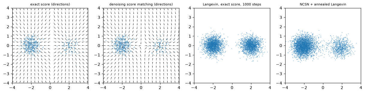
• Plain Langevin gets the weights wrong, even with the perfect score. Each chain falls into the mode nearest its start and crosses the low-density gap very rarely. The score near a mode does not “know” how heavy the other mode is.
• Annealing fixes it. At σ = 3 the blurred density is one broad bump with the right weights, so the chains are distributed correctly before the gap opens.
• A learned noise-conditional network does the same. One network learns all ten blurred scores by denoising — a diffusion model in all but name (§5.1).

8. Continuous time: the VP-SDE (Problem Set 4, problem 3)

As T → ∞ with β_t scaled down accordingly, DDPM’s chain becomes the variance-preserving SDE of Song et al. (2021):

with β_min = 0.1 and β_max = 20.

(a) Marginals. The SDE is linear, so $x(t) \mid x(0)$ is Gaussian with mean $m(t)\, x(0)$ and variance $1 - m(t)^2$, where

For $p(x(0)) = \sum_i \pi_i \mathcal N(\mu_i, \sigma_i^2)$, integrating against the data:

(b) The score. With $v_i = m^2\sigma_i^2 + 1 - m^2$ and responsibilities $r_i(x) \propto \pi_i \mathcal N(x; m\mu_i, v_i)$,

(c) Generation. Anderson’s (1982) reverse-time SDE

run from t = 1 down to 0 has the same marginals in reverse. So does the deterministic probability-flow ODE, $dx = [-\tfrac12\beta x - \tfrac12\beta\, \nabla \log p_t]\, dt$.

Code 07 uses π = (0.6, 0.4), μ = (−2, 1.5), σ = (0.4, 0.3):

• Forward. The simulated forward SDE matches (a) at every t (L1 of 0.03–0.05, histogram noise). At t = 1, m = 0.0066.

• Score. The closed-form score matches a finite-difference derivative of log p_t to three decimals.

• Generation, starting from N(0, 1) with the exact score:

  sampler	steps	L1 to p_data	left fraction (0.60)
  reverse SDE	1000	0.035	0.599
  probability-flow ODE	1000	0.036	0.600
  reverse SDE	30	0.082	0.601
  probability-flow ODE	30	0.051	0.596
  reverse SDE	10	0.329	0.597
  probability-flow ODE	10	0.142	0.590

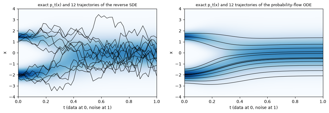
• The score is all the generator needs. Both reverse processes recover the 60 / 40 data exactly with enough steps. The ODE maps each starting noise to one sample deterministically, yet has the same marginals.
• With few steps the ODE degrades more gracefully. The SDE’s injected noise must be removed again by the score term, which first-order steps do poorly. This is why fast samplers (DDIM, DPM-Solver, EDM’s Heun sampler, Lecture 13) integrate the ODE. MIT 6.S184’s notes cover the SDE / ODE view in depth.

9. Many perspectives on diffusion

The slides close with a list, after Sander Dieleman’s blog post “Perspectives on diffusion”. Diffusion models can be read as:

10. Summary

1. Forward process. $x_t = \sqrt{\bar\alpha_t} x_0 + \sqrt{1 - \bar\alpha_t}\varepsilon$, in one jump; variance preserving; the schedule decides how fast signal turns to noise. With β from 1e-4 to 0.02, x_T is pure noise for T ≥ 1000.
2. Reverse process. $q(x_{t-1} \mid x_t)$ is unknown, but $q(x_{t-1} \mid x_t, x_0)$ is a Gaussian with mean $\frac{1}{\sqrt{\alpha_t}}(x_t - \frac{\beta_t}{\sqrt{1-\bar\alpha_t}}\varepsilon)$. One small step back is Gaussian to 10⁻⁷ nats; big jumps toward the data are bimodal.
3. Objective. The variational bound is a sum of noise-L2 terms weighted by λ_t. Setting the weights to 1 favours sample quality: on glyphs FID 33 vs 89, at a worse bound (94 vs 74 nats). Naive ELBO training also suffers from gradient variance, which importance sampling of t removes.
4. Problem Set 4.
   • A latent-space MLP DDPM gives valid 0.90 on glyphs, where the pixel-space MLP gives 0.44.
   • 100 sampling steps are nearly as good as 1000.
   • T = 500 beat T = 1000 with the pset’s schedule, because the noise range mattered, not the step count.
   • The VP-SDE’s marginals and scores are exact, and both the reverse SDE and the ODE regenerate the data.
5. EBMs and scores. $p \propto e^{-E}$; the score $-\nabla E$ needs no Z. Score matching (explicit, sliced, denoising) learns it from samples, and denoising score matching is noise prediction. Langevin dynamics samples with it but mixes poorly between modes; annealing over noise levels fixes that — which is what diffusion does.

11. Common pitfalls

1. “The forward process must be simulated step by step.” It has a closed form for every t (§2.2).
2. “The network learns q(x_{t−1} | x_t, x_0).” That one is known; the network learns the unknown q(x_{t−1} | x_t), using the known one as a regression target (§3).
3. “More diffusion steps are always better.” The range of noise levels matters more than the count (§5.4); and samplers can skip steps (§5.4, Lecture 13).
4. “L_simple is just a crude ELBO.” It is a deliberate reweighting toward sample quality; the ELBO weighting wins on likelihood and loses on samples (§4.4).
5. “Langevin with the true score samples the distribution.” In the limit, yes; in practice it cannot move mass between separated modes (§7.4).
6. “The ODE and the SDE give different distributions.” With the exact score they have the same marginals; they differ in stochasticity and discretization error (§8).

12. Exercises

Exercise 1 (Problem Set 4, 1(a)(b)). Prove $q(x_t \mid x_0) = \mathcal N(\sqrt{\bar\alpha_t}x_0, (1-\bar\alpha_t)I)$. What is $\bar\alpha_T$ for the linear schedule from 1e-4 to 0.02 with T = 1000, approximately, using $\log(1 - \beta) \approx -\beta$?

The proof is in §2.2.

$\log \bar\alpha_T \approx -\sum_t \beta_t = -T \cdot \frac{\beta_{\min} + \beta_{\max}}{2} = -1000 \cdot 0.01005 = -10.05$, so $\bar\alpha_T \approx 4.3 \cdot 10^{-5}$. The exact value is 4.04e-5; the next term of the expansion, $-\beta^2/2$, accounts for the difference.

For T = 500: $\log \bar\alpha_T \approx -5.03$, so $\bar\alpha_T \approx 6.6 \cdot 10^{-3}$ (exact: 6.35e-3).

Exercise 2 (the posterior). Derive $\tilde\mu_t$ and $\tilde\beta_t$ of §3.2 by completing the square, and show the ε form of the mean.

The log of the product, as a function of $x_{t-1}$, is

• Quadratic coefficient: $-\frac12\big(\frac{\alpha_t}{\beta_t} + \frac{1}{1-\bar\alpha_{t-1}}\big)$, giving the precision of §3.2 and hence $\tilde\beta_t$.
• Linear coefficient: $\frac{\sqrt{\alpha_t}x_t}{\beta_t} + \frac{\sqrt{\bar\alpha_{t-1}}x_0}{1 - \bar\alpha_{t-1}}$. Multiplying by $\tilde\beta_t$ gives $\tilde\mu_t$.
• The ε form: substitute $x_0 = (x_t - \sqrt{1-\bar\alpha_t}\varepsilon)/\sqrt{\bar\alpha_t}$. The $x_t$ coefficients add to $\frac{\alpha_t(1 - \bar\alpha_{t-1}) + \beta_t}{(1 - \bar\alpha_t)\sqrt{\alpha_t}} = \frac{1}{\sqrt{\alpha_t}}$. The ε coefficient is $-\frac{\sqrt{\bar\alpha_{t-1}}\beta_t\sqrt{1 - \bar\alpha_t}}{(1 - \bar\alpha_t)\sqrt{\bar\alpha_t}} = -\frac{\beta_t}{\sqrt{\alpha_t}\sqrt{1 - \bar\alpha_t}}$.

Exercise 3 (the ELBO decomposition). Derive the decomposition of §4.1 from $\log \frac{p_\theta(x_{0:T})}{q(x_{1:T} \mid x_0)}$, using $q(x_t \mid x_{t-1}) = q(x_{t-1} \mid x_t, x_0)\, q(x_t \mid x_0) / q(x_{t-1} \mid x_0)$ (the Markov property makes conditioning on $x_0$ free).

The last sum telescopes to $\log q(x_1 \mid x_0) - \log q(x_T \mid x_0)$, which cancels the $q(x_1 \mid x_0)$ and leaves

Take $-\mathbb E_q$ to get $L_T + L_0 + \sum_t L_{t-1}$.

Exercise 4 (the weights). With $\sigma_t^2 = \tilde\beta_t$, show $\lambda_t = \frac{\beta_t}{2\alpha_t(1 - \bar\alpha_{t-1})}$. Why is it largest at small t?

$\lambda_t = \frac{\beta_t^2}{2\tilde\beta_t\alpha_t(1-\bar\alpha_t)}$. Substituting $\tilde\beta_t = \frac{1-\bar\alpha_{t-1}}{1-\bar\alpha_t}\beta_t$ gives $\lambda_t = \frac{\beta_t}{2\alpha_t(1 - \bar\alpha_{t-1})}$.

At small t, $1 - \bar\alpha_{t-1} \approx \sum_{s<t}\beta_s$ is tiny — almost no noise has been added yet — so λ_t is large. For t = 2: $\beta_2/(2\alpha_2\beta_1) \approx 1.2 \cdot 10^{-4}/(2 \cdot 10^{-4}) \approx 0.6$, as code 02 printed. Predicting the noise at nearly clean levels is weighted heavily by the bound, though it changes the image imperceptibly.

Exercise 5 (denoising score matching). Complete the proof in §7.2, including what the “const” is. What is the minimizer of the DSM objective?

Left side: $\mathbb E_{q_\sigma}\|s_\theta\|^2 - 2\mathbb E_{q_\sigma}[s_\theta^\top \nabla\log q_\sigma] + \mathbb E_{q_\sigma}\|\nabla\log q_\sigma\|^2$.

Right side: $\mathbb E_{pq}\|s_\theta\|^2 - 2\mathbb E_{pq}[s_\theta^\top\nabla\log q(\tilde x \mid x)] + \mathbb E_{pq}\|\nabla\log q(\tilde x\mid x)\|^2$.

The first terms are equal (same marginal of $\tilde x$), and the cross terms are equal by the computation in §7.2. So the two sides differ by the constant $\mathbb E_{q_\sigma}\|\nabla\log q_\sigma\|^2 - \mathbb E_{pq}\|\nabla\log q(\tilde x\mid x)\|^2$.

The minimizer over all functions is $s^*(\tilde x) = \mathbb E[\nabla\log q(\tilde x\mid x) \mid \tilde x] = \nabla\log q_\sigma(\tilde x)$, the score of the noised data. That is also “the best noise prediction is $\mathbb E[\varepsilon\mid\tilde x]$” (Tweedie’s formula).

Exercise 6 (Langevin’s stationary distribution). Show that p is stationary for the continuous-time Langevin diffusion $dx = \nabla\log p(x)\, dt + \sqrt 2\, dW$, using the Fokker–Planck equation $\partial_t \rho = -\nabla\cdot(\rho\nabla\log p) + \Delta\rho$.

At ρ = p: $-\nabla\cdot(p\nabla\log p) + \Delta p = -\nabla\cdot(\nabla p) + \Delta p = 0$.

Stationarity says nothing about how fast ρ approaches p. With two modes separated by a low-density gap, the convergence time grows exponentially with the barrier height — code 06’s 0.53 → 0.59 in 10,000 steps.

Exercise 7 (Problem Set 4, 3(a)). Derive m(t) for the VP-SDE from $\frac{d}{dt}\mathbb E[x] = -\frac12\beta(t)\mathbb E[x]$ and the variance equation $\frac{d}{dt}v = -\beta v + \beta$. Show $v(t) = 1 - m(t)^2 + m(t)^2 v(0)$.

Mean. $\mathbb E[x(t)] = \mathbb E[x(0)]\exp(-\frac12\int_0^t\beta) = m(t)\,\mathbb E[x(0)]$, with $\int_0^t\beta(s)ds = \beta_{\min}t + \frac12(\beta_{\max}-\beta_{\min})t^2$.

Variance. $\frac{d}{dt}(v - 1) = -\beta(v - 1)$, so $v(t) - 1 = (v(0) - 1)\,m(t)^2$, i.e. $v(t) = 1 - m(t)^2 + m(t)^2 v(0)$.

For $x(0) = \mu_i$ exactly, v(0) = 0, giving the conditional variance $1 - m^2$. For a component with variance $\sigma_i^2$, $v = 1 - m^2 + m^2\sigma_i^2$, as in §8.

Exercise 8 (hands-on). (a) In 04_ddpm_glyphs.py, predict $x_0$ instead of ε (the network outputs $\hat x_0$; use $\hat\varepsilon = (x_t - \sqrt{\bar\alpha_t}\hat x_0)/\sqrt{1-\bar\alpha_t}$ in the sampler). Compare samples. (b) In 05_ddpm_timesteps.py, try the cosine schedule with T = 1000. (c) In 06_score_matching.py, change the mode weights to 0.95 / 0.05. How many annealing levels does annealed Langevin need to get them right?

(a) x₀-prediction with an unweighted L2 loss emphasizes the noisy levels (where x₀ is hard to predict) differently from ε-prediction; samples are often blurrier. Lecture 13 discusses the v-parameterization as a compromise.

(b) The cosine schedule spends fewer levels at almost-pure noise. Given script 05’s finding, expect it to do at least as well as the linear T = 1000.

(c) The first levels must be broad enough that the blurred density is unimodal with the right weights. With more extreme weights the sampler is more sensitive to the largest σ and to the number of steps per level; expect to need σ₁ ≳ the mode separation and a few more levels.

13. Further reading

From the slides

• J. Sohl-Dickstein et al., Deep Unsupervised Learning using Nonequilibrium Thermodynamics, ICML 2015.
• J. Ho, A. Jain, P. Abbeel, Denoising Diffusion Probabilistic Models, NeurIPS 2020.
• A. Hyvärinen, Estimation of Non-Normalized Statistical Models by Score Matching, JMLR 2005.
• P. Vincent, A Connection Between Score Matching and Denoising Autoencoders, Neural Computation 2011.
• Y. Song, S. Ermon, Generative Modeling by Estimating Gradients of the Data Distribution, NeurIPS 2019.
• Y. Song, D. P. Kingma, How to Train Your Energy-Based Models, arXiv 2021.
• Y. LeCun et al., A Tutorial on Energy-Based Learning, 2006.
• S. Dieleman, Perspectives on diffusion (blog), 2023.

Beyond the slides

• Y. Song et al., Score-Based Generative Modeling through Stochastic Differential Equations, ICLR 2021 (Problem Set 4, problem 3).
• A. Nichol, P. Dhariwal, Improved Denoising Diffusion Probabilistic Models, ICML 2021 (cosine schedule, learned variances, importance sampling of the ELBO).
• T. Salimans, J. Ho, Should EBMs model the energy or the score?, 2021; and Progressive Distillation, ICLR 2022 (Lecture 13).
• B. D. O. Anderson, Reverse-time diffusion equation models, Stochastic Processes and their Applications, 1982.
• MIT6.S184 (in Chinese): flow matching and diffusion through SDEs and ODEs.

Related notes in this course

• Lecture 3 (the ELBO); Lecture 8 §1 (the one-page preview), §2.4 (few-step tightening); Lecture 11 §5 (GANs and score differences).

14. Next lecture

Lecture 13: Diffusion in practice — guidance, distillation and high resolution (reading session · 10/22).

This lecture’s DDPM is unconditional, needs hundreds of steps, and ran on 16×16 glyphs. Lecture 13’s papers address all three:

• classifier-free guidance makes diffusion models follow a condition (and trades diversity for fidelity, like truncation in Lecture 10);
• progressive distillation halves the number of sampling steps again and again;
• simple diffusion shows how to train directly on high-resolution pixels by shifting the noise schedule — the schedule lesson of §5.4, at scale.