Maps to: MIT 6.S978 Deep Generative Models (Fall 2024), Reading · Thu 10/24/2024 · Diffusion beyond Denoising (student paper session). Required papers:
- A. Bansal, E. Borgnia, H.-M. Chu, J. S. Li, H. Kazemi, F. Huang, M. Goldblum, J. Geiping, T. Goldstein, Cold Diffusion: Inverting Arbitrary Image Transforms Without Noise, NeurIPS 2023;
- S. Rissanen, M. Heinonen, A. Solin, Generative Modelling With Inverse Heat Dissipation, ICLR 2023;
- M. Delbracio, P. Milanfar, Inversion by Direct Iteration: An Alternative to Denoising Diffusion for Image Restoration (InDI), TMLR 2023.
Optional: G. Daras, M. Delbracio, H. Talebi, A. G. Dimakis, P. Milanfar, Soft Diffusion: Score Matching for General Corruptions, TMLR 2023.
Basis: This session consisted of student presentations, with no published slides. The notes are organized around the session’s question: does diffusion work because of Gaussian noise, or because of the framework “degrade step by step, restore step by step”? First §1 measures what different degradations do; then each paper in turn; then a side-by-side answer (§6). Paper claims are labelled “the paper reports / argues”. All experiments were designed for these notes and run on a CPU with 16 × 16 glyphs and residual MLP restorers. Two outcomes differed from what I expected and are reported as they came out:
- inverse heat dissipation with the paper’s small training noise (σ = 0.01) was unstable with our MLP; it worked with σ = 0.08, but at low quality;
- in InDI, the best PSNR came at 2 steps rather than 1.
Code:
code/lecture14/— 4 scripts + the shared moduledegradations.py. They run in 2–72 s. Reading time: 3–4 hours including running the code.
0. How to read this lecture
0.1 Where we are
Lectures 12–13 built diffusion models around one specific corruption: adding Gaussian noise. Everything rested on it:
- the closed-form forward process;
- the Gaussian posterior ;
- the ELBO reducing to an L2 loss;
- the score interpretation;
- the SDE/ODE view.
Yet the algorithm — corrupt a little at a time, learn to undo one step, chain the steps — never used Gaussianity in an obvious way. This session’s papers test that separation:
| paper | forward process | what the network predicts | sampler | noise? |
|---|---|---|---|---|
| Cold diffusion | any deterministic degradation : blur, masking, pixelation, … | the clean image | restore, re-degrade (two variants) | none |
| Inverse heat dissipation (IHDM) | the heat equation (blur), plus a little noise | the slightly less blurred image | one step back + fresh noise δ | small, essential |
| InDI | the straight line from the degraded image y to the clean image x | the clean image x | small steps toward the estimate | optional |
| Soft diffusion (optional) | blur and noise together | the clean image | a “momentum” sampler | yes, with a theory of why |
0.2 Learning goals
- Compare degradations by what they leave behind: information about the content, the dimension of the end distribution, and the conditioning of the inverse (§1).
- Explain cold diffusion’s two samplers and why the improved one tolerates restoration errors for linear degradations; explain its diversity problem (§2).
- Derive the heat equation’s solution in the DCT basis; explain the two roles of noise in IHDM: regularizing an ill-posed inverse, and creating diversity (§3).
- Derive InDI’s update, connect one step to the MMSE estimate, and explain the perception–distortion trade-off (§4).
- State soft diffusion’s argument for why noise is needed, and view blur + noise as Gaussian diffusion with frequency-dependent schedules (§5).
- Answer the session’s question (§6).
0.3 Map
| Section | Content | Code |
|---|---|---|
| §1 | What degradations destroy and leave behind | 01_degradations.py |
| §2 | Cold diffusion | 02_cold_diffusion.py |
| §3 | Inverse heat dissipation | 03_heat_dissipation.py |
| §4 | InDI | 04_indi.py |
| §5 | Soft diffusion; blurring diffusion | — |
| §6 | The big picture: what is the noise for? | — |
1. Degradations as forward processes
A forward process has three jobs:
- lead from the data to an end distribution that we can sample;
- do so gradually, so each reverse step is easy;
- keep each reverse step well defined.
Gaussian noise does all three. Code 01 measures what four degradations do on 2000 glyphs, at levels (1 = fully degraded):
- noise: Lecture 13’s cosine schedule;
- blur: the heat equation with blur std from 0.5 to 20 px;
- mask: a growing fixed set of pixels set to 0;
- pixelate: blocks of px.
Content. First, how often the exact Bayes classifier (an empirical prior of 5000 glyphs; Lecture 13 §4.3) still names the right digit:
| level s | noise | blur | mask | pixelate |
|---|---|---|---|---|
| 0.2 | 0.934 | 0.996 | 0.914 | 0.976 |
| 0.4 | 0.900 | 0.954 | 0.904 | 0.961 |
| 0.6 | 0.723 | 0.526 | 0.871 | 0.959 |
| 0.8 | 0.329 | 0.365 | 0.693 | 0.634 |
| 1.0 | 0.105 | 0.271 | 0.105 | 0.278 |
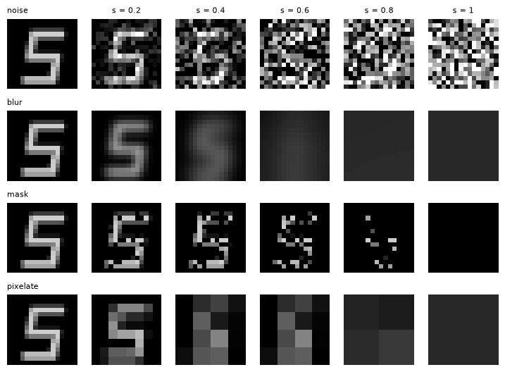
All four erase the digit eventually, along different paths:
- noise drowns the whole image evenly;
- blur keeps the coarse shape (95% at σ_B ≈ 2 px);
- masking keeps the identity until nearly every pixel is gone;
- pixelation keeps it until the blocks are as large as the strokes.
A fully blurred or pixelated glyph is one gray level, and that is still above chance (0.27): the amount of ink says something about the digit.
The end distribution. Second, the effective dimension (participation ratio of the covariance spectrum) of the degraded data:
| level s | noise: dim / variance | blur | mask | pixelate |
|---|---|---|---|---|
| 0 (clean) | 13.5 / 13.2 | 13.5 / 13.2 | 13.5 / 13.2 | 13.5 / 13.2 |
| 0.6 | 196.9 / 46.6 | 1.9 / 0.83 | 11.9 / 5.2 | 5.4 / 3.0 |
| 1.0 | 226.9 / 64.2 | 1.0 / 0.53 | 0.0 / 0.00 | 1.0 / 0.53 |
This is the most important table of the lecture:
- Gaussian noise ends in a full-dimensional distribution, which we can sample exactly and which has as many different points as there are images to generate.
- Deterministic degradations collapse the data. Total blur maps every glyph to a constant image — one number per glyph (mean 0.136, std 0.045). Total masking maps every glyph to the same black image.
A deterministic inverse can therefore produce at most a one-parameter family of images (blur), or a single image (masking). Whatever diversity the samples have must come from somewhere other than the end point.
The inverse. Third, can we just invert the blur? In the DCT basis (§3.1) blur multiplies coefficient by , so the exact inverse divides by it:
| blur σ_B | largest amplification | RMS error of the inverse, no noise (float64) | with noise 1e-3 |
|---|---|---|---|
| 0.61 px | 24.5 | 3e-15 | 5.3e-3 |
| 1.09 px | 2.8e4 | 1.3e-13 | 2.4 |
| 1.95 px | 1.9e14 | 5.5e-4 | 1.1e10 |
The inverse exists mathematically and is useless in practice: an invisible perturbation of 1e-3 is amplified into garbage from σ_B ≈ 1 px on. Deblurring is ill-posed (Lecture 2 §1). A learned restorer cannot compute the lost high frequencies; it must choose plausible ones — it generates.
These three measurements frame the papers: cold diffusion asks whether the step-by-step framework survives without noise; IHDM and soft diffusion explain what noise contributes; InDI uses the framework for restoration, where the end point (the degraded image) is given.
2. Cold diffusion (Bansal et al.)
2.1 The setup
Pick any degradation with and increasing severity in t. Train a restoration network by plain regression:
No noise, no likelihood, no score — “cold”, as opposed to the “hot” Gaussian diffusion. The paper uses blur, inpainting with growing masks, super-resolution, “snowification”, and even “animorphosis” (blending toward an animal photo).
2.2 Two samplers
Starting from :
With a perfect restorer both are exact. The difference is how they treat errors.
Suppose D is linear and , while is still on the true path (Exercise 3):
- Algorithm 1 gives . It hands the next step an image that is the right blur level plus a blurred copy of the error. Such images lie on no true degradation path, and the next restoration starts from an input it was never trained on.
- Algorithm 2 gives . The error enters only through how much its degradation changes between adjacent levels, which is small when the levels are close. Algorithm 2 moves along “the difference between two degradations of the same estimate”. It behaves like DDIM, which also re-uses the current state and moves it by a difference (Lecture 13 §1.3).
2.3 Experiment: restoration
Code 02 trains a residual MLP restorer for blur (20 levels, L1 loss, 31 s). It reconstructs 2000 test glyphs from three blur levels:
| level | sampler | PSNR (dB) | correct digit | valid | FID |
|---|---|---|---|---|---|
| 5 (σ_B 1.1 px) | direct (one step) | 29.2 | 1.000 | 0.990 | 2.6 |
| Algorithm 1 | 25.9 | 0.998 | 0.974 | 4.3 | |
| Algorithm 2 | 29.8 | 1.000 | 0.991 | 2.6 | |
| 10 (σ_B 2.9 px) | direct | 26.4 | 0.994 | 0.966 | 4.2 |
| Algorithm 1 | 19.3 | 0.894 | 0.808 | 16.4 | |
| Algorithm 2 | 26.8 | 0.998 | 0.982 | 3.1 | |
| 15 (σ_B 7.6 px) | direct | 17.8 | 0.521 | 0.707 | 116.7 |
| Algorithm 1 | 14.2 | 0.474 | 0.743 | 80.0 | |
| Algorithm 2 | 17.2 | 0.551 | 0.765 | 73.1 |
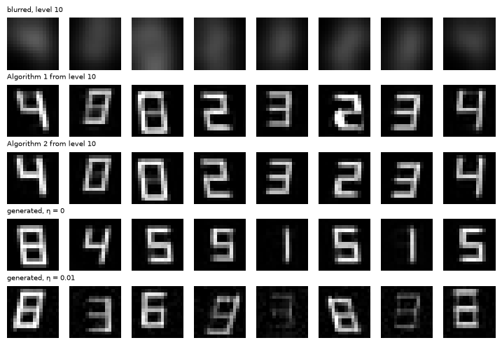
- The paper’s central finding reproduces. At level 10 the naive sampler loses 7.5 dB and a tenth of the digits, and its errors are visible: the figure shows a 0 restored as an 8. Algorithm 2 matches or beats a single direct restoration.
- At level 15 nothing reconstructs the original: script 01 showed the digit is mostly gone. Here the restorers invent: validity stays at 0.7–0.77 while the right digit is found only half the time.
For pixelation (4 levels: blocks of 2, 4, 8, 16 px) Algorithm 2 again gives the most realistic restorations — FID 69 against 156–159 from 8-px blocks. PSNR barely differs (15.5–16.2), because four big levels leave few steps over which errors compound.
2.4 Generation, and the diversity problem
To generate, start from a fully degraded image that no data image produced. For blur, that is a constant gray image. The paper fits a Gaussian mixture to the per-channel means of the training images; we draw the gray level from the 20,000 training means. Then run Algorithm 2 down from level 20:
| start | valid | class entropy (bits) | FID | diversity (real 0.315) |
|---|---|---|---|---|
| exact constant (η = 0) | 0.843 | 2.23 | 474 | 0.185 |
| + noise η = 0.003 | 0.723 | 2.82 | 188 | 0.267 |
| + noise η = 0.01 | 0.664 | 3.15 | 65 | 0.308 |
| + noise η = 0.03 | 0.207 | 3.17 | 69 | 0.326 |
From exact constants, generation is a deterministic function of one number. The glyphs are recognizable, but they form a one-parameter family, and the gray level — the ink amount — picks the digit:
- the darkest starts become 1s (mean gray 0.056), then 4, 9, 5, 6, and the brightest become 8s (0.214);
- 0, 2 and 7 never appear (class entropy 2.2 bits instead of 3.32).
A little noise in the start breaks the symmetry: FID drops seven-fold and all digits appear. But the restorer was never trained on noisy inputs, so validity falls as η grows. The paper discusses the same issue — deterministic degradations give little diversity — and perturbs the starting point to break the symmetry.
2.5 What the paper shows, and its limits
The paper reports:
- restorations and generations for many transforms, all with the same recipe;
- Algorithm 1 failing for most of them and Algorithm 2 working;
- an argument that Algorithm 2 is exact to first order for degradations that change smoothly with t.
Its message is that the step-by-step framework is far more general than Gaussian noise, and that the sampler matters as much as the network.
Its limits are the ones measured above:
- for generation with a deterministic degradation the end distribution is degenerate, so diversity has to be injected by hand;
- nothing in the method is a probabilistic model: there is no likelihood and no guarantee that samples follow the data distribution.
3. Inverse heat dissipation (Rissanen, Heinonen & Solin)
3.1 The heat equation in the DCT basis
The heat equation (with reflecting borders) spreads every pixel’s intensity to its neighbours, conserving the total. Its solution is a Gaussian blur of variance (Exercise 2). In a basis of Laplacian eigenfunctions it is trivial to solve. For an image with reflecting borders those are the discrete cosine transform basis functions:
Every frequency decays independently, the high ones fastest, and the mean () never changes. degradations.heat is these three lines: DCT, multiply, inverse DCT.
The forward process is therefore coarse-to-fine by construction, with a hard ordering of frequencies. It is the deterministic counterpart of Lecture 13 §4.5, where Gaussian noise drowned the frequencies from the top down.
3.2 The model
IHDM defines blur levels for , with blur stds log-spaced from 0.5 px to the image size. It changes two things relative to cold diffusion:
- Training noise. The input is with a small σ, and the network predicts the next, less blurred image: .
- Sampling noise. , with fresh noise at every step and δ slightly larger than σ. The paper uses σ = 0.01, δ = 0.0125.
The Gaussian transitions make IHDM a proper latent-variable model with an ELBO, like DDPM. The prior — essentially the mean colour — is estimated from the training data.
The paper argues that the noise plays two roles:
- It regularizes the inverse. Below the noise level, high-frequency content in the input is indistinguishable from noise, so the network learns to leave it alone rather than amplify it. This is the classical Wiener-filter behaviour: deblur only the frequencies whose SNR is high enough.
- It creates diversity. Fresh noise at step k contains every frequency. The frequencies about to be “un-blurred” are amplified by the next steps into detail. So the noise injected along the way, not the prior, decides most of what is drawn.
3.3 Experiment
Code 03 implements IHDM on glyphs (20 levels, a residual MLP, 32 s per model).
With the paper’s σ = 0.01 the chain is unstable. Each single step is accurate — its error is at the noise level — but chaining them is not:
| start level k | one-step RMS error | RMS error after the whole chain k → 0 | pixel range |
|---|---|---|---|
| 20 | 0.0104 | 0.581 | −2.59 / 3.73 |
| 10 | 0.0125 | 0.217 | −1.05 / 1.82 |
| 5 | 0.0127 | 0.062 | −0.35 / 1.30 |
Generation with δ = 0.0125 gives no valid glyph. The cause is role 1 in reverse. The network sharpens whatever high-frequency content lies above the noise level. Our MLP’s own errors (~0.0125) are above σ = 0.01, so each step’s error is treated as signal by the next step and amplified (script 01: up to -fold per pixel of blur). The paper’s U-Nets are accurate enough for σ = 0.01. Our MLP needs a noise level above its own error.
With σ = 0.08 the chain is stable, and the sampling noise behaves as the paper describes:
| sampling noise δ | valid | class entropy | FID | diversity | diversity from ONE start |
|---|---|---|---|---|---|
| 0 | 0.417 | 1.35 | 681 | 0.103 | 0.027 |
| 0.08 (= σ) | 0.432 | 2.65 | 240 | 0.206 | 0.163 |
| 0.10 (= 1.25σ) | 0.393 | 2.88 | 169 | 0.228 | 0.189 |
| 0.16 (= 2σ) | 0.153 | 3.15 | 89 | 0.277 | 0.248 |
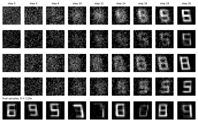
- Without sampling noise the samples are nearly identical (class entropy 1.4 bits). From one starting gray level they are almost exactly the same image (diversity 0.03).
- Diversity comes from the noise along the way, not from the prior. With δ = 1.25σ, 2000 samples from one starting gray level are almost as diverse as samples from all starting levels (0.19 vs 0.23).
- Too much noise hurts validity: the network sees inputs noisier than in training.
- Quality stays low (valid ≈ 0.4; the strokes are often broken). The method works in direction, not in quality, at this scale. The paper reports FIDs on MNIST, CIFAR-10, AFHQ, FFHQ and LSUN churches that are reasonable but not state of the art.
- Generation is visibly coarse to fine. A blob of brightness first, the digit’s layout in the middle of the chain, sharp strokes at the end.
3.4 What the paper reports
The paper emphasizes properties that follow from the explicit frequency ordering:
- Disentanglement of colour and shape. The prior fixes the overall colour, and the chain draws the shapes. Interpolating in the prior changes colour while the noise path keeps the shape.
- Smooth interpolations.
- An inductive bias toward natural-image spectra.
Its broader point is that “noise” in diffusion models can be decomposed: the order in which information is destroyed is a design choice (here explicit, by frequency), and the stochasticity is a separate ingredient.
4. InDI: Inversion by Direct Iteration (Delbracio & Milanfar)
4.1 Restoration, not generation
InDI addresses image restoration: given a degraded image (blurred, compressed, low-resolution, noisy), produce a clean . The classical answer is regression: train with an L2 loss, which gives the posterior mean . When is ambiguous, that mean averages several plausible images — the “regression to the mean” that makes restorations look blurry or ghostly. Diffusion-based restoration (SR3, Palette) samples from instead, but starts from pure noise and needs many steps. InDI keeps the step-by-step idea but starts from itself.
4.2 The iteration
Define a straight path between the clean and the degraded image:
and train for all t. Restore with N equal steps from :
The update has a simple meaning (Exercise 4): with the current estimate , it moves to the point at time on the straight line between and . Each step makes a small move toward the current estimate, and re-estimates from the less degraded image.
- N = 1 is one jump from y to : exactly the regression estimate, for an L2 loss.
- Many steps commit progressively. Early steps fix what is certain. Later steps start from inputs in which an ambiguity has already been half-resolved, so they sharpen toward one plausible answer rather than the average.
4.3 The perception–distortion trade-off
Blau & Michaeli (2018) proved that, for an ambiguous restoration problem, no estimator can be both optimal in MSE and perfectly realistic. The MMSE estimate is unrealistic (an average of images is not an image), and a realistic sample from has twice the MMSE error (Exercise 5). InDI’s step count moves along that trade-off.
Code 04 degrades glyphs with a 3-px blur plus noise of std 0.05 — strong enough that a fifth of the digits are ambiguous — and restores them with one trained InDI network (L2 loss, 33 s):
| restoration | PSNR (dB) | half-tone pixels (real 0.071) | correct digit | valid | FID |
|---|---|---|---|---|---|
| degraded input y | 12.34 | 0.135 | 0.371 | 0.000 | 1755 |
| InDI, N = 1 (regression) | 19.31 | 0.092 | 0.777 | 0.774 | 43.5 |
| N = 2 | 19.41 | 0.087 | 0.781 | 0.822 | 33.0 |
| N = 4 | 19.36 | 0.083 | 0.784 | 0.845 | 23.0 |
| N = 8 | 19.25 | 0.081 | 0.790 | 0.859 | 18.3 |
| N = 32 | 19.04 | 0.079 | 0.786 | 0.864 | 16.1 |
| N = 64 | 18.95 | 0.078 | 0.785 | 0.863 | 14.9 |
(“Half-tone pixels” counts gray values in [0.25, 0.55]: the faint “ghost” segments an average of several candidate digits draws.)
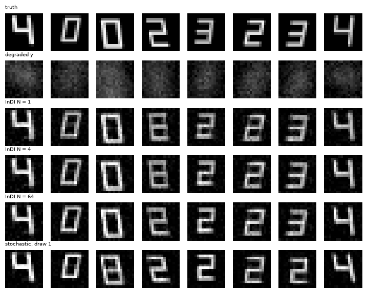
- Regression (N = 1) hedges. Where the digit is ambiguous it draws the disputed segments at partial intensity. The figure shows a 2 restored as a ghostly 8.
- More steps commit. The ghosts fade, validity rises from 0.77 to 0.86, and FID falls three-fold.
- PSNR moves the other way, slightly. After a small gain at N = 2 it declines by half a decibel: a committed guess that is wrong costs more squared error than a hedge.
- The right digit is found equally often at every N (~0.78). The steps change how the glyph is drawn, not what information y contains.
I expected PSNR to peak exactly at N = 1. It peaked at N = 2, because a finite network is not a perfect MMSE estimator. The trend after that is the expected one, and modest in PSNR.
4.4 Adding noise: from one answer to samples
A deterministic restoration returns one answer per input, even when the honest answer is “a 3 or an 8”. The InDI paper discusses adding noise along the path to make the process stochastic. Code 04, Part 2 implements a simple version of my own:
- path: ;
- restoration: redraw the noise at each step.
With N = 32:
- One draw: PSNR 16.84, right digit 0.651, valid 0.857, FID 11.3 (the most realistic restorations), half-tone 0.073.
- Four draws of the same y differ (pixel std 0.030). At least one of them shows the right digit 77.9% of the time; best-of-4 PSNR is 18.31 dB.
A single draw is right less often than the deterministic restoration (0.65 vs 0.79), as it should be. A sample from picks the less likely digit with the probability that digit has. A sampler expresses the ambiguity; the deterministic restorer hides it.
4.5 Where InDI sits
InDI is a flow between two distributions: degraded images at t = 1, clean images at t = 0, connected by straight lines and traversed with a learned field. Lecture 16 meets the same construction for generation (rectified flow; stochastic interpolants between any two distributions), where y is replaced by noise. The paper reports that on real restoration tasks — motion deblurring, JPEG artifact removal, super-resolution, denoising — InDI reaches realistic restorations in a few steps, with the step count as an explicit dial between distortion and perceptual quality.
5. Optional: soft diffusion, and blur as frequency-dependent noise
5.1 Soft diffusion (Daras et al.)
Soft diffusion asks the question this lecture keeps returning to: for a general linear corruption (e.g. = blur), what should the network learn, and why is noise needed?
- Soft score matching. Train to predict , but measure the error after applying the corruption: . The paper shows this learns the score of the corrupted distribution, provided noise is present (). Without noise the corrupted distribution is degenerate — it lives on a lower-dimensional set, exactly §1’s dimension collapse — and has no score.
- The momentum sampler generalizes cold diffusion’s Algorithm 2 to blur plus noise. It moves by the change in degradation between levels, , and adjusts the noise level. It is to soft diffusion what DDIM / ancestral sampling are to Gaussian diffusion.
- The paper reports that blur-plus-noise schedules match or improve on pure noise on small image datasets. It also argues that noise is what makes the method a well-posed generative model: it makes corrupted distributions at neighbouring levels overlap. That is the same reason instance noise rescued GANs in Lecture 11.
5.2 Blurring diffusion = Gaussian diffusion with per-frequency schedules
In the DCT basis, blur plus white noise acts on each coefficient independently (the DCT is orthonormal, so white noise stays white):
i.e. a Gaussian diffusion per frequency, with signal scale and SNR that falls fastest for high frequencies. Hoogeboom & Salimans’ Blurring Diffusion Models (ICLR 2023) make this precise: blurring diffusion is a standard diffusion model in the frequency domain, with a different noise schedule for each frequency. Plain Gaussian diffusion already destroys high frequencies first (Lecture 13 §4.5); blur makes the ordering steeper.
So once noise is added, “diffusion beyond denoising” folds back into Gaussian diffusion with a cleverer schedule. What cannot be folded back is the noise-free case, and §1–§3 measured its costs.
6. The big picture: what is the noise for?
| cold diffusion | IHDM | InDI | Gaussian diffusion (L12–13) | |
|---|---|---|---|---|
| forward path | any deterministic | heat equation + small noise | line from y to x (+ optional noise) | |
| end distribution | degenerate (a constant, a black image) | ≈ degenerate + noise | the given degraded image | full-dimensional N(0, I) |
| network predicts | ε / x / v | |||
| source of diversity | starting point only (hand-perturbed) | noise injected at every step | optional noise | the starting noise and (ancestral) the steps |
| our best generation / restoration | restoration: Alg. 2 matches one-step regression in PSNR, beats it in FID; generation: FID 65–474 | generation: FID 89–681, valid ≤ 0.43 | restoration: FID 43.5 → 14.9 with steps | Lecture 13: FID 3.7 (latent, conditional) |
The answer to the session’s question, as far as these experiments go:
-
The step-by-step framework does not need Gaussian noise for restoration. Cold diffusion’s Algorithm 2 and InDI restore images from blur and pixelation through many small learned steps, and the sampler matters (Algorithm 2 vs 1: 26.8 vs 19.3 dB).
-
For generation, noise does three jobs that deterministic degradations cannot:
- it makes the end distribution full-dimensional and exactly samplable (§1);
- it regularizes the ill-posed inverse, so a chain of imperfect steps stays stable (§3.3);
- it supplies the randomness that becomes diversity (§2.4, §3.3).
Gaussian noise does all three at once, and its coarse-to-fine ordering comes for free (Lecture 13 §4.5).
-
Once noise is added to another degradation, the result is again a Gaussian diffusion, with a different schedule per frequency (§5.2).
What these papers did change is the field’s mental model. The forward process is a design choice. Restoration can start from the degraded image instead of from noise. Straight paths between two distributions (InDI) are a natural object. That last idea becomes flow matching and stochastic interpolants in Lecture 16.
7. Summary
- Degradations differ in what they leave. Noise keeps a full-dimensional end distribution (effective dimension 227); blur and pixelation collapse every glyph to one gray level (dimension 1); masking to one image. Naive inverse blurring amplifies 1e-3 noise into errors of at σ_B ≈ 2 px.
- Cold diffusion. A restorer + the improved sampler restores blurred glyphs well (26.8 dB at level 10 vs 19.3 for the naive sampler). Generation from total blur yields a one-parameter family (class entropy 2.2 bits, FID 474) unless noise is added.
- IHDM. The heat equation is diagonal in the DCT basis. Training noise regularizes the inverse, and sampling noise creates diversity: from one starting gray level, diversity 0.03 without noise vs 0.19 with δ = 1.25σ. With our MLP the paper’s σ = 0.01 was unstable; σ = 0.08 worked at low quality.
- InDI. Walk the straight line from y to x in N steps. N = 1 is regression (best PSNR ±0.1 dB, ghost segments); N = 64 is realistic (FID 14.9 vs 43.5) at −0.5 dB. Noise along the path turns it into sampling.
- Soft diffusion / blurring diffusion. Noise makes general corruptions well posed; blur + noise is Gaussian diffusion with per-frequency schedules.
8. Common pitfalls
- “Blur is invertible, so blur-based generation is easy.” It is invertible only in exact arithmetic; with any noise or model error the inverse is unstable (§1). The restorer must generate the missing frequencies.
- “The naive cold sampler is fine if the restorer is good.” With any error it drifts off the degradation path; Algorithm 2 is far more robust (§2.3).
- “Deterministic degradations give diverse samples if the start is random.” The start of a fully blurred image is one number per image; diversity is limited to a one-parameter family (§2.4).
- “IHDM’s noise is a minor detail.” Without it (or with too little for the network’s accuracy) the reverse chain is unstable, and without sampling noise all samples are alike (§3.3).
- “More InDI steps give better restorations.” More realistic, slightly less accurate in MSE; which is better depends on the use (§4.3).
- “Diffusion beyond denoising replaces Gaussian diffusion.” Every method that generates well here reintroduces noise; with noise, blur becomes a frequency-dependent Gaussian schedule (§5.2).
9. Exercises
Exercise 1 (the DCT diagonalizes the discrete heat equation). For the 1-D discrete Laplacian with reflecting borders, with and , show that is an eigenvector with eigenvalue . Compare with .
Answer
Interior points. Using with and : . So .
Borders. At , the reflection holds because . The same holds at .
Comparison. For small , ; at the highest frequency, , the discrete value is about 4 against . degradations.heat uses the continuous (as IHDM does), so its highest frequencies decay somewhat faster than the discrete heat equation’s.
Exercise 2 (heat = Gaussian blur). Show that the solution of on the line is .
Answer
In Fourier space, , so . The factor is the Fourier transform of a Gaussian with variance , since transforms to . A product in Fourier space is a convolution in space. Hence blur std , as blur_taus uses.
Exercise 3 (why Algorithm 2 tolerates errors). Let D be linear in its image argument, , and . Compute for both algorithms. What happens if D(·, t) changes slowly with t?
Answer
Algorithm 1. .
Algorithm 2. .
When D changes slowly. If changes slowly with t, then , which is small. Algorithm 2’s error per step is the derivative of the degradation of the error, not the degraded error itself. With a perfect restorer (e = 0) both are exact.
Exercise 4 (InDI’s update). Show that is the point at time on the line , if and .
Answer
From : . Substitute:
The bracket simplifies to , giving .
So each step re-estimates and moves to the right point on the straight line between the estimate and y. With it returns .
Exercise 5 (sampling costs twice the MMSE). Let and let be an independent sample from . Show . How many dB of PSNR is that? Compare with code 04.
Answer
Given y, x and x’ are i.i.d. with mean m and covariance Σ, so , while . Doubling the MSE costs dB.
In code 04, one stochastic draw has PSNR 16.84 against 19.31 for regression: 2.5 dB lower. That is close to 3 dB; the draws are approximate samples and the regressor an approximate mean.
Exercise 6 (blur + noise as per-frequency diffusion). With , write the SNR of DCT coefficient k. At blur std 2 px and noise , which frequencies (in cycles per 16 px) still have SNR > 1 for a coefficient of size 1?
Answer
. With and , the condition is , i.e. , i.e. , i.e. .
DCT index k corresponds to k/2 cycles across the image, so roughly 3 cycles per 16 px survive: the strokes’ layout, but not their edges.
Exercise 7 (the dimension argument). Explain why a deterministic sampler started from a fully blurred glyph can produce at most a one-parameter family of images, and why IHDM’s noise escapes this.
Answer
A fully blurred 16 × 16 glyph is a constant image, determined by one number. A deterministic map from into image space traces a curve, so its image is at most one-dimensional.
IHDM injects fresh 256-dimensional noise at each of its 20 steps. The sampler is then a map from to images, which can cover the data’s many directions of variation. Script 03 shows this: with δ = 0, samples from one gray level have diversity 0.03; with δ = 1.25σ, 0.19.
Exercise 8 (hands-on).
(a) In 02_cold_diffusion.py, train the blur restorer with a little input noise (σ = 0.01) and repeat Part 2. Does validity hold up better under start noise?
(b) In 03_heat_dissipation.py, try σ = 0.04. Where is the boundary between a stable and an unstable chain for our MLP?
(c) In 04_indi.py, train with an L1 loss (the paper’s choice for some tasks). What does N = 1 become, and does PSNR still peak at small N?
Answer (sketch)
(a) A restorer that has seen noise treats small perturbations as noise. Expect validity to degrade more slowly with η, at some cost in sharpness at η = 0.
(b) The chain stays stable when σ exceeds the network’s one-step error by a margin: with errors of ~0.0125 expect instability near σ = 0.01–0.02 and stability by ~0.05. Measure one-step RMS errors to locate it.
(c) With L1, one step returns (per pixel) a conditional median rather than the mean, which hedges less. Expect fewer ghost segments at N = 1 and a smaller gap between N = 1 and large N.
10. Further reading
Required papers
- A. Bansal et al., Cold Diffusion: Inverting Arbitrary Image Transforms Without Noise, NeurIPS 2023.
- S. Rissanen, M. Heinonen, A. Solin, Generative Modelling With Inverse Heat Dissipation, ICLR 2023.
- M. Delbracio, P. Milanfar, Inversion by Direct Iteration: An Alternative to Denoising Diffusion for Image Restoration, TMLR 2023.
Optional and related
- G. Daras et al., Soft Diffusion: Score Matching for General Corruptions, TMLR 2023.
- E. Hoogeboom, T. Salimans, Blurring Diffusion Models, ICLR 2023.
- Y. Blau, T. Michaeli, The Perception-Distortion Tradeoff, CVPR 2018.
- C. Saharia et al., Image Super-Resolution via Iterative Refinement (SR3), 2021; Palette: Image-to-Image Diffusion Models, 2022.
Related notes in this course
- Lecture 2 (restoration as inference, ill-posed deblurring); Lecture 11 §4 (instance noise makes distributions overlap); Lecture 13 §4.5 (diffusion is spectral autoregression), §1.3 (DDIM).
11. Next lecture
Lecture 15: Discrete diffusion (reading session · 10/29).
This lecture changed the degradation while keeping continuous pixels. Lecture 15 changes the space: text and tokens are discrete, and there is no Gaussian noise to add. D3PM defines forward processes by transition matrices — uniform resampling, or masking (the absorbing state, which Lecture 8 met as order-agnostic autoregression). DiffuSeq sidesteps discreteness by diffusing word embeddings. SEDD replaces the score by ratios of probabilities. §1’s question returns in a new form: the masking process ends in a single all-[MASK] sequence — a degenerate end point, like total blur — yet masked diffusion generates diverse text. The explanation is that each reverse step samples tokens instead of predicting them deterministically.