Lecture 16 · Flow Matching

Maps to: MIT 6.S978 Deep Generative Models (Fall 2024), Reading · Thu 10/31/2024 · Flow Matching 1 (student paper session). Problem set 5 (released 11/05) belongs here: conditional flow matching on MNIST, ablations of the ODE solver and of the conditional field, and a Gaussian-to-Gaussian flow in 2-D. Required papers:

• Y. Lipman, R. T. Q. Chen, H. Ben-Hamu, M. Nickel, M. Le, Flow Matching for Generative Modeling, ICLR 2023;
• M. S. Albergo, E. Vanden-Eijnden, Building Normalizing Flows with Stochastic Interpolants, ICLR 2023;
• X. Liu, C. Gong, Q. Liu, Flow Straight and Fast: Learning to Generate and Transfer Data with Rectified Flow, ICLR 2023.

Optional: T. Fjelde, E. Mathieu, V. Dutordoir, An Introduction to Flow Matching (Cambridge MLG blog, 2024).

Basis: This session consisted of student presentations, with no published slides. The notes are organized around one question — can we learn the velocity field of a flow from noise to data directly, by regression, without simulating it? — and the three papers that answered it at the same time, in three different languages. Background the papers rely on (continuous normalizing flows, the continuity equation) comes first. Paper claims are labelled “the paper reports / proves”. All experiments were designed for these notes and run on a CPU. Most use 2-D Gaussian mixtures, for which the marginal velocity field is known exactly, so learned fields, losses and samplers can be compared with the truth. The last experiments use the glyph latents of Lecture 12. Several outcomes differed from what I expected and are reported as they came out:

• the linear (“OT”) path’s marginal trajectories are more bent than the cosine path’s, yet easier to integrate;
• all three standard paths turned out to define the same map from noise to data;
• distilling the reflowed coupling into one step was no easier than distilling the original one;
• a bridge between two multimodal data sets failed without a little extra noise.

Code: code/lecture16/ — 6 scripts + the shared module flow_matching.py. They run in 10–95 s. Reading time: 4–5 hours including running the code.

0. How to read this lecture

0.1 Where we are

Lectures 12–13 arrived at a deterministic sampler for diffusion models: DDIM, which Lecture 13 §5 showed to be Euler’s method on an ODE, the probability-flow ODE. That ODE moves noise to data, and a network trained to denoise defines its velocity. This lecture turns the order around:

• Diffusion fixes a noising process, learns to undo it, and then discovers that the result can be written as an ODE.
• Flow matching starts from the ODE. It chooses how probability mass should travel from noise to data (a probability path), and regresses a network directly on the velocity of that travel.

The three papers of this session found this idea independently in 2022:

They are three descriptions of one algorithm. The differences that matter in practice are which path, which time weighting and which sampler. Lecture 17 scales the algorithm up (Stable Diffusion 3, SiT).

0.2 Learning goals

1. Explain why maximum-likelihood training of continuous normalizing flows is expensive, and what flow matching avoids (§1).
2. Derive the marginal velocity from conditional ones (Theorem 1), and prove that the conditional loss has the same gradient (Theorem 2). Explain the loss floor (§2.1–2.3).
3. Derive the conditional field of a Gaussian path; write the OT and diffusion paths; solve Pset 5’s Gaussian-to-Gaussian problem (§2.4).
4. Show that all affine Gaussian paths define the same flow up to a change of clock and scale, and say what a path choice changes instead (§2.5).
5. Convert between velocity, score and denoiser; build a bridge between two non-Gaussian distributions (§3).
6. State rectified flow’s guarantees (marginals preserved, transport cost non-increasing), and explain reflow, straightness and distillation (§4).
7. Compare ODE solvers by function evaluations, fixed and adaptive (§5).

0.3 Notation and time direction

In this lecture time runs from noise ($t = 0$) to data ($t = 1$), as in all three papers and Pset 5:

Lectures 12–13 used the opposite direction ($t = 0$ data). So do SD3 and SiT in Lecture 17. Always check a paper’s convention before copying a formula.

0.4 Map

1. Background: continuous normalizing flows

1.1 A flow defined by an ODE

Lecture 4 built normalizing flows from a stack of invertible layers. Take the limit of infinitely many infinitesimal layers and you get an ordinary differential equation:

The flow $\phi_t$ maps a starting point $x_0$ to where the ODE has carried it by time t. If v is smooth, $\phi_t$ is invertible (run the ODE backwards). It pushes $p_0$ forward to a distribution $p_t$. A network $v_\theta$ in place of v gives a continuous normalizing flow (CNF; Chen et al. 2018). Any network architecture is allowed, because invertibility comes from the ODE, not from the layers.

1.2 How the density moves

Two equivalent descriptions.

Along a trajectory (the instantaneous change of variables):

It is the continuous version of Lecture 4’s log-determinant: where the field spreads out (positive divergence), density drops.

At a fixed point (the continuity equation, conservation of mass):

The rate at which mass at x changes equals the net flow of mass into x. We say that v generates the probability path $(p_t)$. Code 01 checks this equation numerically for its exact field (relative residual $10^{-9}$–$10^{-8}$).

1.3 Why training CNFs was expensive

Maximum likelihood needs $\log p_1(x)$ for each data point x:

1. integrate the ODE backwards from x to $x_0$;
2. accumulate $\int\nabla\!\cdot v\,dt$ along the way, using trace estimators in high dimension (FFJORD, Grathwohl et al. 2019);
3. backpropagate through the whole solver.

Every training step simulates the ODE. The cost grows with the number of solver steps, which itself grows as training makes the field more complex. CNFs were elegant and slow, and they did not scale to large images.

Diffusion models (Lecture 12) escaped this with a simulation-free objective: noise a data point in closed form, regress a denoiser. Flow matching brings the same trick to CNFs.

1.4 The idea in one sentence

If we knew a velocity field $u_t$ that generates a path from $p_0$ = noise to $p_1$ = data, we could just regress on it:

No ODE is solved during training. The rest of §2 shows how to get a usable $u_t$.

2. Flow matching (Lipman et al.)

2.1 Build the path from conditional paths

Writing down $p_t$ and $u_t$ directly is hopeless: $p_1$ is the unknown data distribution. Lipman et al.’s move is to build the path one data point at a time:

• For each data point $x_1$, choose a simple conditional path $p_t(x\mid x_1)$: $p_0(x\mid x_1) = \mathcal N(0, I)$ at $t = 0$, and a tiny blob around $x_1$ at $t = 1$.
• Choose a conditional velocity $u_t(x\mid x_1)$ that generates it. For Gaussian paths it is known in closed form (§2.4).
• Mix over the data:

The marginal velocity is the posterior average of the conditional velocities: all data points $x_1$ whose conditional path could have produced x at time t, weighted by how likely that is.

Theorem 1 (Lipman et al.). If each $u_t(\cdot\mid x_1)$ generates $p_t(\cdot\mid x_1)$, then $u_t$ generates $p_t$.

Proof. Differentiate the mixture, use the conditional continuity equations, and pull the divergence out of the integral:

At $t = 1$ the mixture of tiny blobs is (nearly) the data distribution. So the ODE with velocity $u_t$, started from noise, ends at the data.

2.2 Why the marginal trajectories do not cross

A conditional path is simple. With the “OT” path of §2.4, a pair $(x_0, x_1)$ travels in a straight line. But the lines of different pairs cross. Through a point x at time t pass many lines, heading to different data points.

The ODE cannot follow all of them: it has one velocity per point. Its velocity is their average, and the marginal trajectories therefore never cross. Code 01 draws both pictures for Pset 5’s Gaussian-to-Gaussian problem:

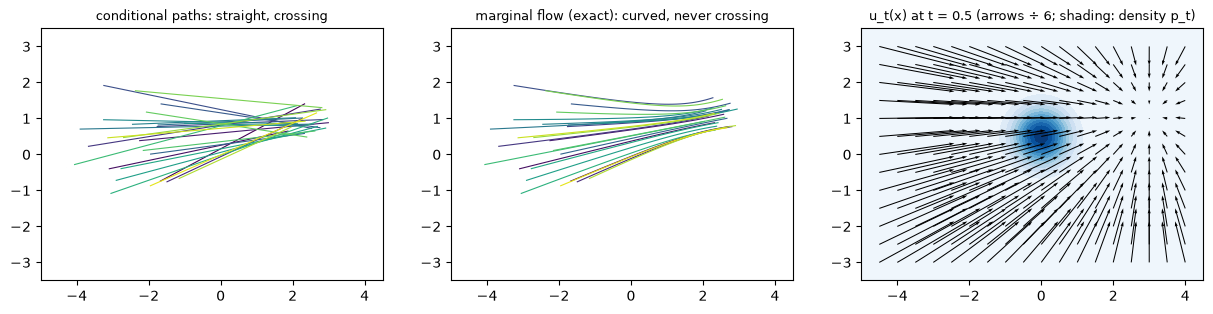
Averaging has a visible cost: even when every conditional path is straight, the marginal trajectories bend (§2.4, §4).

2.3 Conditional flow matching: the same gradient without $u_t$

$u_t$ still involves the unknown $q$. The conditional flow matching loss uses only the conditional field:

Theorem 2 (Lipman et al.). $\mathcal L_{\text{CFM}}(\theta) = \mathcal L_{\text{FM}}(\theta) + C$, where C does not depend on θ. Hence the gradients are equal.

Proof. Expand both squares. The $\lVert v_\theta\rVert^2$ terms are identical, because $x\sim p_t$ in both. The cross terms are equal because $u_t$ is the posterior mean of $u_t(x\mid x_1)$:

What remains does not involve θ. $\square$

The constant is the variance of the conditional target around its mean, $C = \mathbb E\lVert u_t(x\mid x_1) - u_t(x)\rVert^2$. It is the same mechanism that made Lecture 12’s denoising score matching equal to explicit score matching.

Code 02 computes both losses on the ring of 8 Gaussians, where $u_t$ is known exactly (exact_velocity), for networks at four stages of training:

The constant itself is 3.454. Three practical consequences:

• The CFM loss curve flattens far above zero. The trained model’s loss (3.47) is almost all constant. Its level says little about the model; only the small excess does.
• The noise is in the gradient. Over 100,000 samples the two gradients point the same way (cosine 0.999). On a 256-sample minibatch, the CFM gradient has about 8 times the variance of an exact-target gradient (relative variance 0.79 vs 0.10).
• The price is efficiency, not correctness. Trained for the same 4000 steps on the exact target, the model’s field is 10 times more accurate ($\mathcal L_{\text{FM}}$ 0.0015 vs 0.015; sample quality 0.98 vs 0.96). In practice the exact target is never available.

Where the floor sits in t. With the linear path, the conditional target is $x_1 - x_0 = (x_1 - x_t)/(1 - t)$. Its variance given $x_t$ is the uncertainty about $x_1$, magnified by $1/(1-t)^2$:

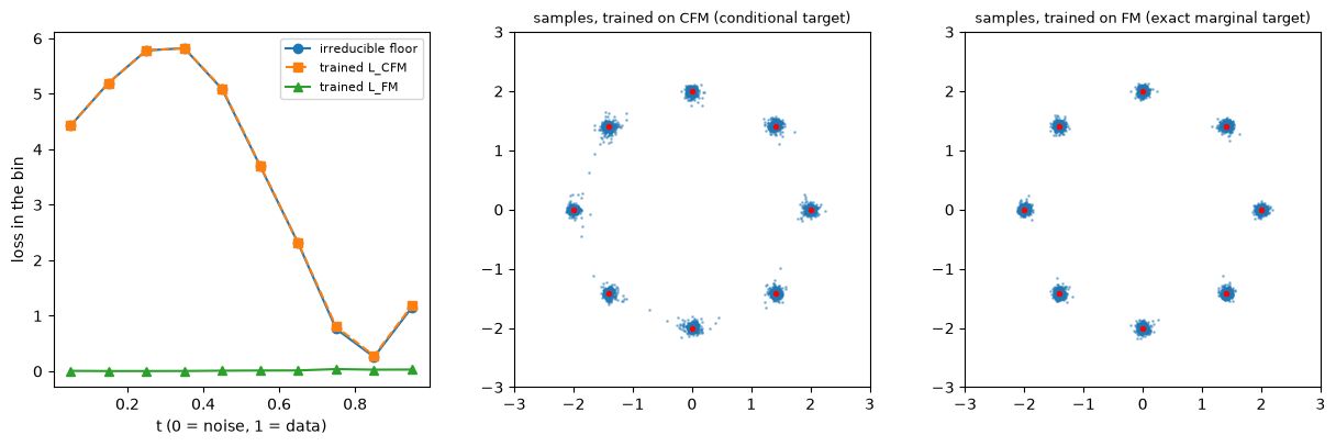
• At $t = 0$: $\mathrm{tr}\,\mathrm{Cov}(x_1) \approx 4$.
• It rises to 5.8 around $t = 0.3$: $x_1$ is still uncertain and the magnification grows.
• It collapses once $x_t$ reveals the mode (0.26 for $t\in[0.8, 0.9]$).
• It rises again to $\mathrm{tr}\,\mathrm{Cov}(x_0) = 2$ at $t = 1$, where $x_1$ is known but the starting noise is not (Exercise 7).

The trained CFM loss tracks this floor in every bin. The model’s real error is largest for $t > 0.7$, where the 8 narrow modes form.

2.4 Gaussian conditional paths

The general form. Take $p_t(x\mid x_1) = \mathcal N(\mu_t(x_1), \sigma_t(x_1)^2 I)$, with $\mu_0 = 0, \sigma_0 = 1$ (noise) and $\mu_1 = x_1$, $\sigma_1 = \sigma_{\min}$ small. The simplest map that pushes $\mathcal N(0, I)$ along it is $\psi_t(x_0) = \sigma_t x_0 + \mu_t$. Its velocity, written at the point $x = \psi_t(x_0)$, is the conditional vector field (Lipman et al., Theorem 3; Exercise 1):

The CFM loss then becomes a regression on a quantity computed from $(x_0, x_1)$ alone, with $x = \psi_t(x_0)$:

The OT path (Pset 5, problem 1). $\mu_t = t x_1$ and $\sigma_t = 1 - (1 - \sigma_{\min})t$:

Lipman et al. call it the OT path because the conditional flow between two Gaussians, $\mathcal N(0, I)$ and $\mathcal N(x_1, \sigma_{\min}^2 I)$, is the optimal-transport displacement: a straight line at constant speed. Pset 5 uses $\sigma_{\min} = 0$, which gives the target $x_1 - x_0$. This is rectified flow’s target too (§4).

Diffusion paths. Lipman et al. also write the paths of score-based models in this form.

• VP (Song et al.’s variance-preserving SDE, read backwards): $\mu_t = \alpha_{1-t}x_1$ and $\sigma_t = \sqrt{1-\alpha_{1-t}^2}$, with $\alpha_s = e^{-\frac12\int_0^s\beta}$ and β from 0.1 to 20. The path does not quite start at pure noise: $\alpha_1 = 0.0066$.
• VE: $\mu_t = x_1$, with $\sigma_t$ growing toward the noise end.

Flow matching can train on any of them; diffusion is then one particular choice of path, trained with a different loss weighting (§6).

Pset 5, problem 3: Gaussian to Gaussian. Source $\mathcal N(\mu_0, \sigma_0^2 I)$, target $\mathcal N(\mu_1, \sigma_1^2 I)$, straight lines $x_t = (1-t)x_0 + t x_1$ between independent end points. Then $x_t$ and $x_1 - x_0$ are jointly Gaussian, and the marginal velocity is a linear regression (Exercise 3):

Code 01 ($\mu_0 = (-2.5, 0)$, $\sigma_0 = 1$; $\mu_1 = (2.5, 1)$, $\sigma_1 = 0.3$) finds:

• The formula is right. It matches the general Gaussian-mixture code to $2\cdot10^{-15}$ and satisfies the continuity equation.
• The end points are optimal. The flow sends every $x_0$ to $\mu_1 + \frac{\sigma_1}{\sigma_0}(x_0 - \mu_0)$, to $5\cdot 10^{-11}$. That is the optimal-transport map between the two Gaussians, and the transport cost equals $W_2^2 = 26.98$; independent pairs cost 28.18.
• The route is not. The intermediate distributions are narrower than the OT interpolation: their std at $t = 0.5$ is 0.52 instead of 0.65, because averaging independent end points shrinks the spread. So the trajectories bend (straightness S = 0.25, defined in §4).
• CFM learns it from samples. A small network trained for 3000 steps (4 s) is within 1–2% of $u_t$ at every t. From the same noise, its samples land on average 0.04 away from the exact flow’s.

2.5 Which path? All affine paths are one flow

Code 03 puts three paths side by side on the ring, first with their exact marginal fields, so that no network error interferes:

Mean end-point error of Euler with N uniform steps:

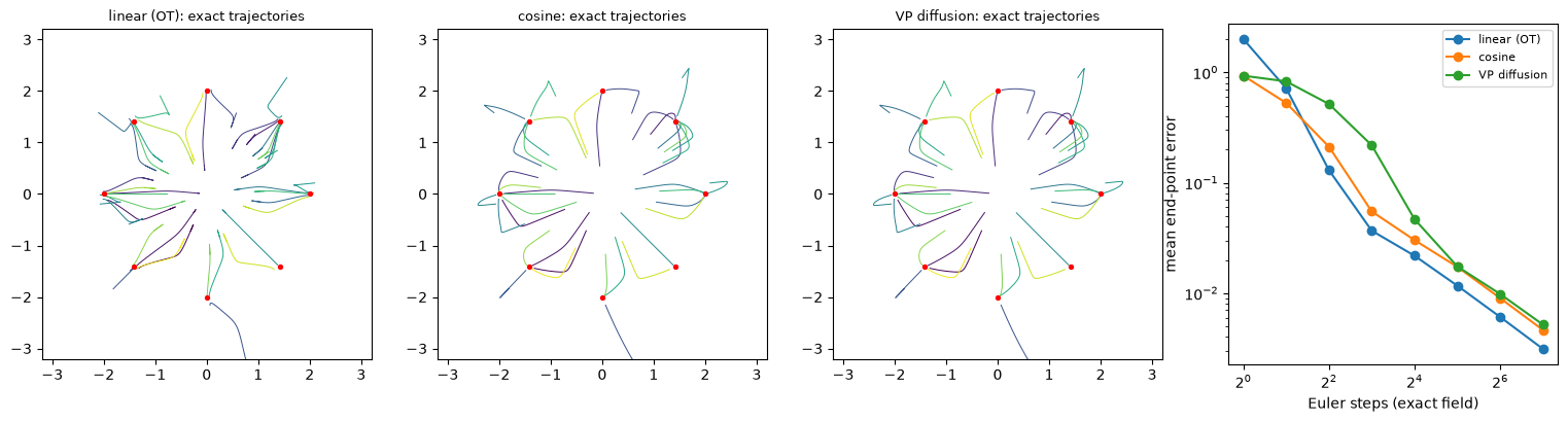
The surprise: one map from noise to data. Run from the same noise, the three exact flows end at the same points: linear vs cosine to $3\cdot 10^{-9}$, and vs VP to $5\cdot10^{-6}$ (VP starts at $a_0 = 0.0066$, not 0). The reason is a short argument.

• Two affine paths $x^A_t = a_t x_1 + b_t x_0$ and $x^B_\tau = \alpha_\tau x_1 + \beta_\tau x_0$ with the same signal-to-noise ratio, $a_t/b_t = \alpha_\tau/\beta_\tau$, are the same random variable up to a factor: $x^A_t = c\,x^B_\tau$ with $c = a_t/\alpha_\tau = b_t/\beta_\tau$.
• This holds pair by pair, so the conditional velocities transform the same way. So do their posterior averages, the marginal velocities. A trajectory of one flow, rescaled by $c(t)$ and run on the clock $\tau(t)$, is a trajectory of the other (Exercise 5).
• At $t = 0$ and $t = 1$ both paths sit at $x_0$ and $x_1$ unscaled ($c = 1$), so the end-point maps coincide.

The cosine and VP paths are both variance-preserving ($a^2 + b^2 = 1$), so $c \equiv 1$, and their trajectories coincide even as curves (same length ratio, 1.232). The linear path’s states are the variance-preserving ones shrunk by $\sqrt{t^2 + (1-t)^2}$ (0.71 at $t = 0.5$), which pulls its trajectories inward: they are the most bent.

So the choice of an affine Gaussian path does not change what the exact flow computes. It changes two things:

1. How hard the ODE is for a solver with a given time grid. What matters to Euler is how much the velocity changes along the way. That is smallest for the linear path (5.1) and largest for VP (9.4), three quarters of which comes after $t = 0.75$: the VP path’s $a_t$ stays near 0 until $t \approx 0.5$ ($a_{0.3} = 0.08$), then everything happens at once. With uniform steps, the linear path is the most accurate from 4 steps on, and dopri5 needs the fewest evaluations there. Liu et al.’s straightness S, which favours the cosine path, did not predict this ranking.
2. What the network must learn, and how the loss weights each time. The regression targets differ in scale and noise; script 03’s learned models show it (below).

One step is a special case. The first Euler step only knows $\mathbb E[x_1\mid x_0] = \mathbb E[x_1]$, the data mean (Exercise 6):

• the linear path moves every sample to the centre of the ring (error 2.0, the ring’s radius);
• the cosine and VP paths start with zero velocity and do not move at all.

No choice of path makes few-step sampling work for multimodal data; that needs straight marginal trajectories (§4).

With learned fields (same network and 4000 training steps per path), the linear path gives the best samples at small step counts. With 4 Euler steps its quality is 0.58, against 0.25 for cosine and 0.03 for VP. From 16 steps on, linear and cosine are equal. dopri5 needs 55 evaluations for these two models and 79 for the VP model. The VP model also ends lower (0.90 vs 0.96 at 100 steps), probably because its targets are largest and noisiest near $t = 1$, exactly where its field changes fastest.

What the paper reports. Lipman et al. train the same U-Net with the OT and the diffusion (VP) path and sample with dopri5 at tolerance $10^{-5}$:

The paper also reports DDPM at 3.12 / 7.48 / 274 on CIFAR-10, and that FM-OT needs roughly 60% of the evaluations of the diffusion models to reach the same numerical error. Our toy ordering — same quality family, fewer evaluations for the OT path — is the same.

3. Stochastic interpolants (Albergo & Vanden-Eijnden)

3.1 Interpolate samples, not densities

Albergo & Vanden-Eijnden start from an interpolant between samples of two arbitrary densities $\rho_0$ and $\rho_1$:

Their main example is the trigonometric interpolant $I = \cos(\frac{\pi t}{2})x_0 + \sin(\frac{\pi t}{2})x_1$: our cosine path. The distribution $\rho_t$ of $x_t$ interpolates between the two densities. The paper proves that it is transported by the velocity

and that v is the unique minimizer of a quadratic objective, $G(\hat v) = \mathbb E\big[\lVert\hat v_t(x_t)\rVert^2 - 2\,\partial_t I\cdot\hat v_t(x_t)\big]$. Up to a constant this is the CFM loss with target $\partial_t I$; the “stochastic” in the title refers to the random end points.

Same algorithm, different emphasis. Compared with Lipman et al.:

• No Gaussian is needed at either end. $\rho_0$ can be any data set (§3.3).
• The paper bounds $W_2(\rho_1, \hat\rho_1)$ by the training objective (times a factor exponential in the Lipschitz constant of $\hat v$).
• It links interpolants to optimal transport. A max-min over interpolants yields the Benamou–Brenier optimal transport; the authors leave the consequences to future work.

The paper reports a CIFAR-10 NLL of 2.99 bits/dim (FID 10.27) and ImageNet-32 NLL 3.48 (FID 8.49), with likelihoods computed by the ODE as for any CNF. It also reports training at 128 × 128, previously out of reach for maximum-likelihood ODE flows.

3.2 A velocity model is a score model

When $\rho_0 = \mathcal N(0, I)$ and $I = a_t x_1 + b_t x_0$, two linear equations link the posterior means $E_1 = \mathbb E[x_1\mid x_t = x]$ and $E_0 = \mathbb E[x_0\mid x_t = x]$:

Eliminate $E_1$, then apply Tweedie’s formula for the Gaussian component ($\nabla\log p_t = -E_0/b_t$, Lecture 12 §7.2):

For the linear path this reads $\nabla\log p_t(x) = \frac{t\,v - x}{1 - t}$. Velocity, score, denoiser $\hat x = E_1$ and noise prediction $\hat\varepsilon = E_0$ are one object in four units (Exercise 4). That is why a flow-matching network can drive the SDE samplers of diffusion models (SiT, Lecture 17).

Code 06, Part 1 checks the formula with exact fields: the score from the velocity matches the true score to $10^{-15}$ for all three paths. For a learned linear-path model the conversion multiplies the velocity error by $t/(1-t)$:

Near the noise end the score is mostly the known Gaussian part $-x/(1-t)$, so even a poor velocity gives a good score. Near the data the factor reaches 19, and score-based samplers inherit the amplified error.

3.3 Bridges between two data sets

Code 06, Parts 2–3 transport the ring of 8 Gaussians to the 5 × 5 grid of 25 Gaussians with the linear interpolant. Training uses the same regression as before, and there is no Gaussian anywhere:

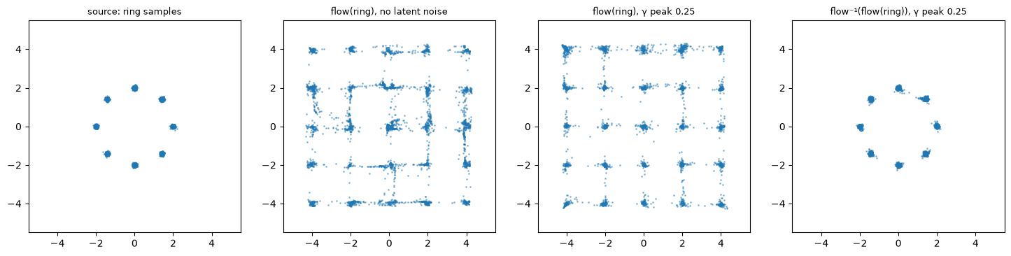
• The bridge works and is invertible. Run backwards from its own output, the flow returns the ring (8 modes, quality 0.96). Liu et al. use exactly this for unpaired image-to-image transfer (cat → wild animal faces) and domain adaptation.
• But it was harder than starting from noise (21 of 25 modes, twice the evaluations). I did not expect this. Each ring mode is a tiny blob (std 0.05) whose mass must fan out to several grid modes, so near $t = 0$ the field must change direction within 0.05. That is hard to learn and stiff to integrate.
• The follow-up paper’s latent noise fixes it. Albergo, Boffi & Vanden-Eijnden (2023, Stochastic Interpolants: A Unifying Framework for Flows and Diffusions) add noise to the interpolant: $x_t = (1-t)x_0 + tx_1 + \gamma(t)z$, with $\gamma(0) = \gamma(1) = 0$. The end points are unchanged, and the target becomes $x_1 - x_0 + \dot\gamma(t)z$. With $\gamma$ peaking at 0.25 all 25 modes appear, the solver needs fewer evaluations, and the round trip is three times more accurate. The noise smooths the intermediate densities.
• Too much noise hurts again (peak 1.0, quality 0.56): the intermediate distribution forgets the source’s structure.

4. Rectified flow (Liu, Gong & Liu)

4.1 Straight lines and couplings

Liu et al. phrase the problem as transport between $\pi_0$ (noise, or any distribution) and $\pi_1$ (data). Given a coupling, i.e. pairs $(X_0, X_1)$, independent at first, train

and define the rectified flow $dZ_t = v(Z_t, t)\,dt$, $Z_0 = X_0$. This is CFM with the linear path, $\sigma_{\min} = 0$. The paper proves two properties:

• Marginals are preserved (Theorem 3.3): $Z_t$ has the same distribution as $X_t$ for every t, so $Z_1\sim\pi_1$. The flow’s pairs $(Z_0, Z_1)$ are a new coupling, now deterministic.
• Transport costs do not increase (Theorem 3.5): $\mathbb E\,c(Z_1 - Z_0)\le\mathbb E\,c(X_1 - X_0)$ for every convex cost c. The proof is two applications of Jensen’s inequality (Exercise 8): once over time along a trajectory, and once over the pairs whose average defines v.

Because the flow never crosses itself, it “rewires” the crossing straight lines into non-crossing paths between nearby partners. Code 04 measures it on the ring. The exact flow’s coupling costs $\mathbb E\lVert Z_1 - Z_0\rVert^2 = 1.02$; independent pairs cost 6.07.

4.2 Straightness

$S = 0$ exactly when every trajectory is a straight line traversed at constant speed. Then one Euler step is exact: $Z_1 = Z_0 + v(Z_0, 0)$. The 1-rectified flow is not straight, because the marginal velocity averages crossing lines (§2.2). On the ring S = 1.5, and one Euler step sends everything to the centre (Exercise 6).

4.3 Reflow

Draw fresh noise $Z_0$, run the trained flow to get $Z_1$, and train a new flow on straight lines between these pairs. This is the 2-rectified flow; repeat for k. The new pairs barely cross: each $Z_0$ was already sent to a nearby $Z_1$. So there is little left to average, and the new flow is straighter. Code 04 trains on 50,000 pairs per round, each round starting from the previous weights, as the paper does:

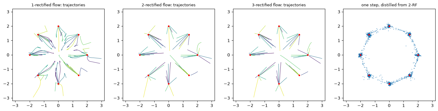
• One reflow straightens almost completely (S 1.52 → 0.002). With a single Euler step, the 2-rectified flow covers all 8 modes with quality 0.85, where the 1-rectified flow produced nothing.
• The transport cost decreases, slightly (1.018 → 1.008 → 1.005), as Theorem 3.5 promises.
• Errors accumulate. Each round learns from the previous model’s samples, so the many-step quality drops (0.957 → 0.951 → 0.938).

The paper reports the same pattern on CIFAR-10. One Euler step gives FID 378 for the 1-rectified flow, 12.21 for the 2-rectified and 8.15 for the 3-rectified. With an adaptive RK45 solver the FID gets worse with each round (2.58, 3.36, 3.96), while the number of evaluations falls (127, 110, 104).

4.4 Distillation

A deterministic coupling is a function $Z_0\mapsto Z_1$. A network can regress it directly: $Z_1 \approx Z_0 + v(Z_0, 0)$ (Liu et al. §2.3). Code 04, Part 3:

• Distillation beats the reflowed flow’s own single step (0.90 vs 0.85).
• The reflowed coupling was no easier to distill. I expected it to be: the paper reports one-step FID 4.85 after 2-rectified + distillation against 6.18 for 1-rectified + distillation. Here the two are equal, and the transport costs explain why. Reflow barely changed the coupling (1.018 vs 1.008); it straightened the paths between nearly the same pairs. Distillation only sees the pairs.

In 2-D the 1-rectified coupling is already a simple function. For images it apparently is not, and reflow simplifies it. The paper’s own framing: distillation approximates the existing coupling, while rectification produces a new one with lower transport cost.

Lecture 18 meets the same goal — one-step generation from a flow — with consistency models, and InstaFlow (Liu et al. 2024) scales reflow + distillation to Stable Diffusion.

5. Sampling: solvers and function evaluations

5.1 The solver zoo

Sampling a flow means solving $\dot x = v_\theta(x, t)$ from $t = 0$ to 1. Cost is counted in NFE, the number of network evaluations.

“Order p” means the error shrinks like $h^p$ once the step h is small. Code 05, Part 0 measures every order on a test ODE with a known solution: Euler 1.01, Heun 1.98, RK4 4.01, and 3.04 and 5.13 for the solutions of bosh3 and dopri5, which also checks their Butcher tableaus.

Adaptive solvers choose their own steps from a tolerance: they take large steps where the field is smooth and small ones where it changes fast. Lipman et al. sample with dopri5 at tolerance $10^{-5}$. Pset 5 asks to compare dopri8, bosh3, fehlberg2 and adaptive_heun (torchdiffeq’s names; dopri8 is not implemented here).

5.2 Pset 5 on glyphs

Code 05 trains CFM (OT path, $\sigma_{\min} = 0$) on Lecture 12’s 64-dimensional glyph latents: 6000 steps, 26 s. The model is cached for Lecture 18. It is then sampled from the same 2000 noise vectors with 16 solver settings:

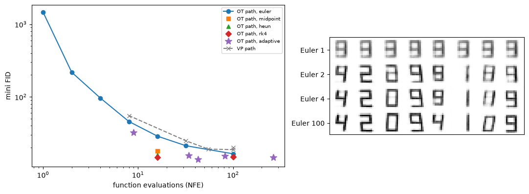
• One step returns a blurred average glyph (FID 1463), the posterior mean of §2.5. Quality rises steeply to ~16–32 evaluations, then saturates near FID 14–16. Beyond that the model’s error, not the solver’s, limits the samples: dopri5 with 265 evaluations is no better than with 43.
• At an equal budget of 16 evaluations, higher order pays. RK4 with 4 steps gives FID 14.7 against 28.8 for Euler with 16 steps. Lecture 13 found the opposite for Heun at ≤ 17 evaluations with an exact diffusion denoiser. The flow here is smooth enough that the higher-order methods’ assumptions hold.
• A tolerance is not a guarantee. Fehlberg 2 stopped after 9 evaluations with poor samples. An adaptive pair estimates its error by the difference between its two formulas. Fehlberg 2’s nominally first-order companion is, at practical step sizes, more accurate than the second-order solution (Part 0: 2.2e-5 vs 8.1e-5 with 20 steps on the test ODE). So the difference understates the error of the solution actually used, and the solver takes steps that are too large.

Pset 5’s second ablation: the diffusion conditional field. The same network trained on the VP path is worse at every setting:

The VP model is not only harder to integrate; it is a worse model, as in code 03. This is the same ordering as Lipman et al.’s table in §2.5.

6. Flow matching and diffusion: one family

Put Lectures 12–13 and this lecture side by side, with both written in the same time direction:

Everything in the left column has a counterpart on the right.

• The paths are the same family. VP diffusion is one affine Gaussian path, and by §2.5 every affine path defines the same exact flow up to clock and scale.
• The predictions are interconvertible (§3.2; Lecture 13 §1.2).
• The losses differ only in how they weight noise levels. Kingma & Gao (2023) write the common diffusion objectives, the flow-matching one included, as weightings of one denoising loss across noise levels (and, for monotonic weightings, as the ELBO of augmented data).

What actually differs between a “diffusion model” and a “flow-matching model” in practice is a bundle of choices: path, target, time sampling, solver. Lipman et al.’s OT path, Albergo’s trigonometric interpolant and Liu’s rectified flow each pick one bundle, and Lecture 17 shows how much each choice matters at scale. Gao et al.’s blog post Diffusion Meets Flow Matching: Two Sides of the Same Coin (2024) makes the equivalence explicit. MIT6.S184 Lecture 2 (in Chinese) derives flow matching from the ODE / SDE side.

7. Summary

1. Flow matching regresses a network on a velocity field that generates a path from noise to data. No simulation is needed during training.
2. Conditional → marginal. The marginal velocity is the posterior average of simple conditional velocities (Theorem 1). CFM regresses on the conditional ones and has the same gradient (Theorem 2). The loss floor (3.45 on the ring) is the conditional target’s variance, and minibatch gradients are ~8× noisier than with the exact target.
3. Gaussian paths. The conditional field is $u = \frac{\dot\sigma}{\sigma}(x - \mu) + \dot\mu$. The OT path gives the target $x_1 - (1-\sigma_{\min})x_0$. Between two Gaussians the flow realizes the OT map at the end points but bends in between.
4. All affine Gaussian paths define the same flow up to clock and scale. Paths differ in how easily solvers integrate them (linear best; VP’s changes pile up near the data) and in how well networks learn them.
5. Stochastic interpolants. Any two distributions, any interpolant. Velocity ↔ score by two linear equations. Data-to-data bridges benefit from a little latent noise.
6. Rectified flow. It preserves marginals and does not increase convex transport costs. Reflow straightens (S 1.52 → 0.002 in one round), enabling one-step sampling, at the price of accumulated error. Distillation turns a coupling into a one-step generator.
7. Solvers. Quality saturates at ~16–40 evaluations on glyphs. RK4 with 4 steps matches dopri5. Adaptive tolerances can mislead (Fehlberg 2).

8. Common pitfalls

1. “The CFM loss should go to zero.” It plateaus at the conditional target’s variance; only the excess over that floor measures the model (§2.3).
2. “The OT path gives straight trajectories.” Its conditional paths are straight. The marginal trajectories bend whenever the data are not a single Gaussian (§2.2, §2.5); straight marginal trajectories need reflow or distillation.
3. “Different paths learn different generative models.” With exact fields, affine Gaussian paths define the same noise-to-data map (§2.5). They differ in learnability and integrability.
4. “More solver accuracy, better samples.” Beyond ~40 evaluations, model error dominates (§5.2). And adaptive solvers only control their own error estimate (Fehlberg 2).
5. “Reflow is free.” Each round trains on generated samples and accumulates error; the paper’s RK45 FIDs get worse with every round (§4.3).
6. “Flow matching needs a Gaussian source.” Any source works (§3.3). Gaussian noise does make the flow’s job easier, and latent noise in the interpolant helps bridges.
7. Time direction. Flow-matching papers use t = 0 for noise, diffusion papers t = 0 for data. Formulas copied across without flipping t produce nonsense.

9. Exercises

Exercise 1 (the conditional field of a Gaussian path). Let $\psi_t(x_0) = \sigma_t x_0 + \mu_t$. Show that the velocity of $\psi_t(x_0)$, written as a function of the current point $x = \psi_t(x_0)$, is $u_t(x\mid x_1) = \frac{\dot\sigma_t}{\sigma_t}(x - \mu_t) + \dot\mu_t$. Specialize it to the OT path.

$\frac{d}{dt}\psi_t(x_0) = \dot\sigma_t x_0 + \dot\mu_t$. Invert the map: $x_0 = (x - \mu_t)/\sigma_t$. Substitute to get the formula.

OT path. $\mu_t = tx_1$, $\sigma_t = 1 - (1-\sigma_{\min})t$, so $\dot\sigma_t = -(1-\sigma_{\min})$ and

The last step puts both terms over the common denominator; the $tx_1$ terms cancel.

Exercise 2 (Theorem 2 in full). Prove that $\nabla_\theta\mathcal L_{\text{CFM}} = \nabla_\theta\mathcal L_{\text{FM}}$, and identify the constant C. Where does the assumption $p_t(x) > 0$ enter?

$\mathcal L_{\text{FM}} = \mathbb E_{p_t}\big[\lVert v\rVert^2 - 2\langle v, u_t\rangle + \lVert u_t\rVert^2\big]$ and $\mathcal L_{\text{CFM}} = \mathbb E_{q, p_t(\cdot\mid x_1)}\big[\lVert v\rVert^2 - 2\langle v, u_t(\cdot\mid x_1)\rangle + \lVert u_t(\cdot\mid x_1)\rVert^2\big]$.

• First terms. Equal: the marginal of x is $p_t$ in both.
• Cross terms. Equal by the definition of $u_t$ as the posterior average. Its definition divides by $p_t(x)$, hence the assumption $p_t(x) > 0$.
• Last terms. Do not involve θ.

So $C = \mathbb E\lVert u_t(x\mid x_1)\rVert^2 - \mathbb E\lVert u_t(x)\rVert^2 = \mathbb E\lVert u_t(x\mid x_1) - u_t(x)\rVert^2$, the variance of the conditional target (law of total variance).

Exercise 3 (Pset 5, problem 3a). Derive the marginal velocity of §2.4 for the Gaussian-to-Gaussian problem.

The joint distribution. $x_t = (1-t)x_0 + tx_1$ and $D = x_1 - x_0$ are jointly Gaussian (linear in independent Gaussians), per coordinate:

• $\mathbb E x_t = m_t$ and $\mathrm{Var}\,x_t = s_t^2 = (1-t)^2\sigma_0^2 + t^2\sigma_1^2$;
• $\mathbb E D = \mu_1 - \mu_0$;
• $\mathrm{Cov}(D, x_t) = \mathrm{Cov}(x_1 - x_0, (1-t)x_0 + tx_1) = t\sigma_1^2 - (1-t)\sigma_0^2$.

The regression. For jointly Gaussian variables, $\mathbb E[D\mid x_t] = \mathbb E D + \frac{\mathrm{Cov}(D, x_t)}{\mathrm{Var}\,x_t}(x_t - m_t)$.

A check. The flow is $x_t = m_t + \frac{s_t}{\sigma_0}(x_0 - \mu_0)$. Its velocity, $\dot m_t + \frac{\dot s_t}{s_t}(x - m_t)$, matches the formula because $s_t\dot s_t = t\sigma_1^2 - (1-t)\sigma_0^2$. At $t = 1$ it gives the OT map $\mu_1 + \frac{\sigma_1}{\sigma_0}(x_0 - \mu_0)$.

Exercise 4 (one object, four units). For the path $x_t = a x_1 + b x_0$ with Gaussian $x_0$, express $\hat x_1 = \mathbb E[x_1\mid x_t]$, $\hat x_0$ and the score in terms of the velocity v. Show that the velocity MSE equals $(\dot a - a\dot b/b)^2$ times the $\hat x_1$-MSE.

The conversions. From $x = a\hat x_1 + b\hat x_0$ and $v = \dot a\hat x_1 + \dot b\hat x_0$:

The MSE. Substitute $\hat x_0 = (x - a\hat x_1)/b$ into v:

Two velocity predictions at the same x differ by $(\dot a - a\dot b/b)$ times the difference of their $\hat x_1$, so the squared errors scale by its square.

For the linear path. The factor is $1 + t/(1-t) = 1/(1-t)$. The velocity loss weights the $\hat x_1$-error by $1/(1-t)^2$, heavily toward the data end: yet another weighting of the same denoising problem (Lecture 13 Exercise 3).

Exercise 5 (affine paths are reparameterizations). Let paths A and B satisfy $a_t/b_t = \alpha_{\tau(t)}/\beta_{\tau(t)}$, and let $c(t) = b_t/\beta_{\tau(t)}$. Show that if $Z^B$ solves B’s marginal ODE, then $Z^A_t = c(t)\,Z^B_{\tau(t)}$ solves A’s, and that the two flows have the same end-point map.

Pathwise relation. For each pair, $x^A_t = a_t x_1 + b_t x_0 = c(t)(\alpha_\tau x_1 + \beta_\tau x_0) = c\,x^B_\tau$. Differentiating: $\partial_t x^A_t = \dot c\,x^B_\tau + c\,\dot\tau\,\partial_\tau x^B_\tau$.

Take conditional expectations. Given $x^A_t = x$, equivalently $x^B_\tau = x/c$:

The trajectory. $Z^A_t = cZ^B_\tau$ satisfies $\dot Z^A = \dot c Z^B + c\dot\tau u^B_\tau(Z^B)$. Since $Z^B = Z^A/c$, this is exactly $u^A_t(Z^A)$, so $Z^A$ solves A’s ODE.

The end points. At $t = 0$: $a = \alpha = 0$ and $b = \beta = 1$, so $c = 1$ and $\tau = 0$. At $t = 1$: $b = \beta = 0$ and $a = \alpha = 1$, so $c = 1$ (by $c = a/\alpha$) and $\tau = 1$. Hence $Z^A_1 = Z^B_1$ from the same $Z_0$.

Code 03 confirms it to $3\cdot10^{-9}$.

Exercise 6 (one Euler step). For the linear path with $\sigma_{\min} = 0$ and a Gaussian source independent of the data, show that one Euler step from $x_0$ gives $\mathbb E[x_1]$. What does it give for the cosine path?

Linear path. $x_0 + u_0(x_0)$, with $u_0(x) = \mathbb E[x_1 - x_0\mid x_0 = x] = \mathbb E[x_1] - x$ by independence. So the step lands at $\mathbb E[x_1]$ for every starting point: the centre of the ring (code 03’s error 2.0), or the average glyph (code 05’s FID 1463).

Cosine path. $\dot a_0 = \pi/2$ and $\dot b_0 = 0$, so $u_0(x) = \frac{\pi}{2}\mathbb E[x_1\mid x_0] = \frac{\pi}{2}\mathbb E[x_1]$. That is 0 for centred data: the step does not move. Either way, one step from a non-straight flow cannot produce samples.

Exercise 7 (the floor at the ends). For the linear path, show that the CFM floor $\mathbb E\lVert(x_1 - x_0) - u_t(x_t)\rVert^2$ equals $\mathrm{tr}\,\mathrm{Cov}(x_1)$ at $t = 0$ and $\mathrm{tr}\,\mathrm{Cov}(x_0)$ at $t = 1$.

At t = 0. $x_t = x_0$ and $u_0 = \mathbb E[x_1] - x_0$, so the residual is $x_1 - \mathbb E x_1$, with variance $\mathrm{tr}\,\mathrm{Cov}(x_1)$ (≈ 4 on the ring).

At t = 1. $x_t = x_1$ and $u_1 = x_1 - \mathbb E[x_0\mid x_1] = x_1 - \mathbb E x_0$ by independence. The residual is $-(x_0 - \mathbb E x_0)$, with variance $\mathrm{tr}\,\mathrm{Cov}(x_0) = d = 2$.

Code 02’s first and last bins: 4.43 and 1.15. Bins average over a range of t; the last bin covers the dip just before $t = 1$.

Exercise 8 (reflow does not increase transport costs). Prove $\mathbb E\,c(Z_1 - Z_0)\le\mathbb E\,c(X_1 - X_0)$ for convex c, using Theorem 3.3 (equal marginals).

Jensen over time. $Z_1 - Z_0 = \int_0^1 v(Z_t, t)\,dt$, so $c(Z_1 - Z_0)\le\int_0^1 c(v(Z_t, t))\,dt$.

Jensen over pairs. $v(z, t) = \mathbb E[X_1 - X_0\mid X_t = z]$, so $c(v(z, t))\le\mathbb E[c(X_1 - X_0)\mid X_t = z]$.

Combine. Take expectations and use that $Z_t$ and $X_t$ have the same distribution:

Equality requires both Jensen steps to be tight: straight trajectories, and no averaging over different directions. That is a fixed point of reflow.

Exercise 9 (hands-on). (a) In 03_paths.py, sample the VP model with Euler on a grid uniform in log-SNR instead of in t. How much of its gap to the linear path closes? (b) In 04_reflow.py, generate the reflow pairs with the exact 1-rectified flow instead of the learned one. Does the 100-step quality still drop across rounds? (c) In 05_glyph_solvers.py, add Euler on a grid that is denser near $t = 1$ (e.g. $t_i = 1 - (1 - i/N)^2$). Does Euler with 8 steps improve?

(a) Code 03 traced most of the VP path’s handicap to its velocity changes piling up after t = 0.75. A grid that follows the signal-to-noise ratio spreads the steps evenly over those changes, so expect a large part of the gap to close. It will not reach the linear path, though: the learned VP field is also less accurate.

(b) With exact pairs the 2-rectified flow trains on the true coupling, so the inherited error disappears. The remaining drop is the reflow network’s own fitting error.

(c) The glyph flow’s velocity changes fastest near the data, where the modes form; a quadratic grid puts more steps there. Expect a visible gain at 8 steps and little at 100.

10. Further reading

Required papers

• Y. Lipman, R. T. Q. Chen, H. Ben-Hamu, M. Nickel, M. Le, Flow Matching for Generative Modeling, ICLR 2023.
• M. S. Albergo, E. Vanden-Eijnden, Building Normalizing Flows with Stochastic Interpolants, ICLR 2023.
• X. Liu, C. Gong, Q. Liu, Flow Straight and Fast: Learning to Generate and Transfer Data with Rectified Flow, ICLR 2023.

Optional

• T. Fjelde, E. Mathieu, V. Dutordoir, An Introduction to Flow Matching (Cambridge MLG blog), 2024 — Pset 5’s Gaussian-to-Gaussian figure follows its Figures 11–12.

Background and follow-ups

• R. T. Q. Chen, Y. Rubanova, J. Bettencourt, D. Duvenaud, Neural Ordinary Differential Equations, NeurIPS 2018; W. Grathwohl et al., FFJORD, ICLR 2019 (CNFs trained by maximum likelihood).
• M. S. Albergo, N. M. Boffi, E. Vanden-Eijnden, Stochastic Interpolants: A Unifying Framework for Flows and Diffusions, 2023 (latent noise $\gamma(t)z$; ODE and SDE samplers).
• A. Tong et al., Improving and Generalizing Flow-Based Generative Models with Minibatch Optimal Transport, TMLR 2024 (OT couplings within minibatches instead of reflow).
• X. Liu et al., InstaFlow: One Step is Enough for High-Quality Diffusion-Based Text-to-Image Generation, ICLR 2024 (reflow + distillation for Stable Diffusion).
• D. Kingma, R. Gao, Understanding Diffusion Objectives as the ELBO with Simple Data Augmentation, NeurIPS 2023; R. Gao et al., Diffusion Meets Flow Matching: Two Sides of the Same Coin (blog), 2024.
• Y. Lipman et al., Flow Matching Guide and Code, 2024 (a comprehensive tutorial with a reference library).

Related notes in this course

• Lecture 4 (discrete normalizing flows); Lecture 12 (Tweedie, the probability-flow ODE); Lecture 13 §1 (parameterizations) and §5 (DDIM = Euler, EDM samplers); MIT6.S184 Lecture 2 (in Chinese).

11. Next lecture

Lecture 17: Scaling flow matching, and discrete flow matching (reading session · 11/05).

This lecture established that path, target, time weighting and sampler are separate choices around one regression. Lecture 17 asks which choices matter at scale:

• Stable Diffusion 3 trains rectified flows with time samplers that favour the middle of the path (logit-normal), a two-stream Transformer (MM-DiT), and a resolution-dependent shift of t — Lecture 13’s simple-diffusion shift in flow language.
• SiT separates interpolant, prediction target and ODE vs SDE sampling on a DiT backbone, and measures each.
• Discrete flow matching carries probability paths and velocities over to tokens, where masking (Lecture 15) reappears as one path among many.