Maps to: MIT 6.S978 Deep Generative Models (Fall 2024), Reading · Thu 09/26/2024 · AR and Tokenizers (student paper session). Required papers:
- L. Yu et al., Language Model Beats Diffusion — Tokenizer is Key to Visual Generation (MAGVIT-v2), ICLR 2024;
- K. Tian, Y. Jiang, Z. Yuan, B. Peng, L. Wang, Visual Autoregressive Modeling: Scalable Image Generation via Next-Scale Prediction (VAR), NeurIPS 2024;
- Q. Yu et al., An Image is Worth 32 Tokens for Reconstruction and Generation (TiTok), 2024.
Optional:
- M. Chen et al., Generative Pretraining from Pixels (iGPT), ICML 2020;
- A. Ramesh et al., Zero-Shot Text-to-Image Generation (DALL·E), ICML 2021;
- F. Mentzer, D. Minnen, E. Agustsson, M. Tschannen, Finite Scalar Quantization: VQ-VAE Made Simple (FSQ), ICLR 2024.
Basis: This session consisted of student presentations, with no published slides. These notes are organized around the question the papers share — “autoregressive models need discrete units; how should an image be cut into tokens, how many, from how large a vocabulary, in which order?” Numbers from the papers are labelled “the paper reports” and given only where the claim is central. All experiments were designed for these notes and run on a CPU with GlyphWorld images, reusing Lecture 3’s tokenizer pieces. Several outcomes contradicted my plan — next-scale prediction lost on quality at our scale; LFQ needed a much larger entropy weight — and are reported as they came out. Code:
code/lecture07/— 4 scripts + the shared moduletokenizers.py. They run in 50–100 s. Reading time: 4 hours including running the code.
0. How to read this lecture
0.1 Where we are
Lectures 5 and 6 modeled images pixel by pixel. That is exact and simple, but expensive:
- A 256×256 RGB image is 196,608 sub-pixels — 196,608 sequential sampling steps.
- Each conditional must learn both low-level texture and high-level structure.
- Lecture 6 found that small pixel models get the texture and miss the structure.
The modern answer is a two-stage pipeline:
- a tokenizer compresses an image into a short sequence of discrete tokens — Lecture 3’s VQ-VAE, grown up;
- a generative model of the tokens (an autoregressive Transformer, or a masked one) learns their joint distribution. A sample is a token sequence, and the tokenizer’s decoder turns it back into pixels.
This is how DALL·E, Parti, MaskGIT, MAGVIT, VAR and LlamaGen work. Language models handle text the same way, with a text tokenizer (BPE) in place of the image tokenizer.
The papers of this session show that the tokenizer is not a detail. It decides:
- how good images can possibly be (the reconstruction ceiling);
- how hard the generative model’s job is (sequence length, vocabulary size, redundancy);
- what order generation can take (raster, coarse-to-fine, or no spatial order at all).
0.2 Learning goals
- Explain the two-stage pipeline, and separate the tokenizer’s ceiling from the prior’s errors.
- Compare three quantizers — VQ (learned codebook), FSQ (rounded scalars), LFQ (signs) — in mechanism, codebook usage and failure modes (dead codes, unvisited codes), and say what each trick fixes (restarts, entropy loss).
- Explain the vocabulary trade-off: a bigger codebook improves reconstruction but makes the prior’s distribution harder to learn.
- Describe VAR’s multi-scale residual tokenizer and next-scale prediction, the block-causal mask, and the price of predicting a whole scale at once.
- Describe TiTok’s 1-D tokenizer: why latent tokens that are not tied to positions can be far fewer, and why that helps generation.
- Place iGPT, DALL·E and FSQ in this picture.
0.3 Map
| Section | Content | Code |
|---|---|---|
| §1 | From pixels to tokens: iGPT, DALL·E, the two-stage pipeline | 02_token_ar.py |
| §2 | Quantizers: VQ, FSQ, LFQ (MAGVIT-v2) | 01_quantizers.py |
| §3 | The vocabulary trade-off: “the tokenizer is key” | 02_token_ar.py |
| §4 | VAR: next-scale prediction | 03_next_scale.py |
| §5 | TiTok: 1-D tokens | 04_one_d_tokens.py |
| §6 | The big picture | — |
0.4 Data and metrics
Gray GlyphWorld images: 20,000 for training, up to 2,000 for testing. Tokenizers use Lecture 3’s patch encoder and decoder: 16 tokens on a 4×4 grid, each reading an 8×8 window. Generated or reconstructed images are scored by Lecture 3’s Judge:
| metric | real glyphs |
|---|---|
| recognizable | 1.000 |
| valid | 0.989 |
| class entropy | 3.32 bits |
| mini FID | 1.1 |
| nearest-real distance | 0.064 |
A token sequence of length T over a vocabulary of K codes can describe at most T·log₂K bits.
1. From pixels to tokens
1.1 iGPT: GPT on pixels
image GPT (Chen et al. 2020) took a GPT-2-style Transformer and trained it, unchanged, to predict pixels in raster order. To make sequences manageable it:
- downsampled images to 32×32 (up to 64×64);
- replaced each RGB value by one of 512 colour clusters found by k-means — a crude, fixed “tokenizer”.
Even then sequences were 1024–4096 long, and the cost of attention grows with the square of the length. The paper’s main point was representation learning: the features learned by pixel prediction were strong enough for linear classifiers. The lesson for generation: pixels are too many and too small to be good tokens.
1.2 DALL·E: learn the tokens first
DALL·E (Ramesh et al. 2021) separated the two jobs:
- A discrete VAE compresses a 256×256 image into a 32×32 grid of tokens from a vocabulary of 8192 (trained with a Gumbel-softmax relaxation instead of a straight-through estimator). That is 1024 tokens instead of 196,608 sub-pixels.
- A 12-billion-parameter Transformer models the concatenation of up to 256 text tokens (BPE) and the 1024 image tokens, autoregressively.
Text-conditional generation is then just continuing a sequence that starts with the caption. The paper sampled many candidates and reranked them with CLIP.
Every later autoregressive image model keeps this division of labour. The tokenizer handles perception (what details matter, how to compress them); the Transformer handles composition (which tokens go together).
1.3 Experiment: a prior turns a tokenizer into a generator
Lecture 3 ended with “a tokenizer is not a generator”: random tokens decode to garbage, and a bigram prior over Lecture 3’s VQ tokens reached only valid 0.052, FID 166. Code 02 trains a small causal Transformer (2 layers, width 64) on the 16 tokens of each training glyph. Its samples are decoded by the tokenizer. For a codebook of 256 codes:
| valid | FID | |
|---|---|---|
| decoded real tokens (the tokenizer’s ceiling) | 0.978 | 2.1 |
| decoded sampled tokens (Transformer prior) | 0.506 | 27.2 |
| decoded bigram samples (Lecture 3) | 0.052 | 166 |
The prior is where the generative modeling happens. The two rows separate the blame: the gap between real images and the first row is the tokenizer’s, the gap between the two rows is the prior’s.
2. Quantizers: VQ, FSQ and LFQ
2.1 Three ways to make a vector discrete
All three sit between an encoder (continuous vectors z) and a decoder, and pass gradients through the discrete step with the straight-through estimator (Lecture 3 §7.3):
-
VQ (VQ-VAE, Lecture 3): a learned codebook of K vectors; each z is replaced by its nearest code. It needs a codebook loss (pull codes toward encoder outputs) and a commitment loss (pull encoder outputs toward codes). Its failure mode is dead codes: codes that are never anyone’s nearest neighbour never get a gradient. Remedies include restarts (move dead codes onto real encoder outputs), lower-dimensional lookups, and codebook EMA updates.
-
FSQ (finite scalar quantization, Mentzer et al.): project z to a few dimensions (say 4), squash each into a bounded range, and round each dimension to one of L levels. The codebook is the grid of all combinations, Π_i L_i codes (e.g. 8·5·5·5 = 1000). Nothing is learned in the quantizer — no codebook, no auxiliary losses, nothing to die. The paper reports that it matches VQ in MaskGIT-style generators with near-full codebook usage.
-
LFQ (lookup-free quantization, MAGVIT-v2): each dimension becomes its sign, ±1. With d dimensions the implicit codebook is {−1, +1}^d, 2^d codes. The “lookup” is d independent sign tests, so even 2^18 = 262,144 codes cost nothing.
Without help, an encoder uses only a few corners of the hypercube, so MAGVIT-v2 adds an entropy loss on soft assignments p(code | z):
The first term pushes each token to commit to one code; the second pushes the batch as a whole to spread over all codes.
2.2 Experiment: how many codes are actually used?
Code 01 trains the same grid tokenizer with each quantizer at four codebook sizes (1500 steps each). Each cell is RMSE / codes used / perplexity; perplexity is the “effective number” of codes, exp of the entropy of their usage.
| K (bits / image) | VQ + restarts | FSQ | LFQ (entropy weight 0.5) |
|---|---|---|---|
| 16 (64) | 0.080 / 16 / 10.9 | 0.087 / 16 / 13.1 | 0.095 / 16 / 14.7 |
| 64 (96) | 0.060 / 64 / 45.3 | 0.065 / 64 / 40.0 | 0.083 / 63 / 47.3 |
| 256 (128) | 0.052 / 254 / 166 | 0.058 / 238 / 81 | 0.076 / 235 / 108 |
| 1024 (160) | 0.049 / 973 / 526 | 0.055 / 697 / 230 | 0.070 / 720 / 337 |
(A continuous autoencoder with the same encoder and decoder reaches RMSE 0.026.)
- Diminishing returns. Each doubling of K adds one bit per token, but the error falls more and more slowly, and a growing share of the codebook is used rarely (perplexity / K falls).
- VQ with restarts reconstructs best at every size. Its codes move to where the encoder outputs are, while FSQ’s grid points and LFQ’s hypercube corners are fixed, and the encoder must learn to land on them. I had expected FSQ to match VQ; at our scale it did not quite.
- LFQ spends exactly one bit per dimension, so at equal K it needs the widest latent and reconstructs worst on these glyphs. Its advantage is the free lookup for enormous K, which our experiment does not reach.
Without the tricks (K = 1024):
| tokenizer | codes used | perplexity | RMSE |
|---|---|---|---|
| VQ without restarts | 86 | 55.9 | 0.058 |
| VQ + restarts | 973 | 526 | 0.049 |
| LFQ, no entropy loss | 4 | 3.4 | 0.123 |
| LFQ, entropy weight 0.1 (the paper’s value) | 8 | 5.9 | 0.102 |
| LFQ, entropy weight 0.5 | 720 | 337 | 0.070 |
- VQ collapses without restarts (8% of the codebook in use), the dead-code problem of Lecture 3.
- LFQ’s codes cannot die, but they can go unvisited. Without the entropy loss the encoder uses 4 corners of a 10-dimensional hypercube, and reconstructions suffer.
- The entropy weight needs tuning. With the paper’s weight 0.1 it was barely better at our scale; 0.5 opened the codebook. The weight that works depends on the codebook and batch sizes.
3. The vocabulary trade-off: “the tokenizer is key”
3.1 MAGVIT-v2’s claim
MAGVIT-v2’s title states its thesis: with a good enough tokenizer, a language-model-style generator beats diffusion models. Its contributions:
- LFQ, which allows a huge vocabulary (2^18) with near-full usage;
- a tokenizer shared by images and video (a causal 3-D CNN), so that the first frame is tokenized like an image;
- a careful study of how vocabulary size affects both reconstruction and generation.
The paper reports a striking contrast. With VQ, increasing the vocabulary improves reconstruction, but generation quality first improves and then degrades. With LFQ, both keep improving up to very large vocabularies. Its generator is a MaskGIT-style masked Transformer, not a left-to-right one, so “language model” here means “a Transformer over discrete tokens”. The paper reports lower FIDs on ImageNet than the diffusion models it compares against.
3.2 Experiment: bigger codebooks, worse samples
Code 02 measures the trade-off with VQ tokenizers and the same small prior:
| K | max bits / image | ceiling (real tokens): valid / FID | AR samples: valid / FID | AR test NLL (bits / image) |
|---|---|---|---|---|
| 16 | 64 | 0.912 / 11.3 | 0.648 / 26.1 | 23.8 |
| 256 | 128 | 0.978 / 2.1 | 0.506 / 27.2 | 54.0 |
| 1024 | 160 | 0.981 / 1.6 | 0.334 / 39.2 | 75.6 |
- The ceiling improves monotonically with K; the samples get worse. With 16 codes the reconstructions are coarse, but each image is a short, low-entropy description the prior learns easily. With 1024 codes the reconstructions are almost perfect, but each token is a 1-of-1024 choice. The prior must learn a far larger distribution from the same 20,000 images: its NLL triples and its samples degrade.
- This is MAGVIT-v2’s observation for VQ, reproduced in miniature. “The tokenizer is key” because it fixes both the ceiling and the difficulty of the prior. A larger vocabulary pays off only when the prior has the data and capacity to learn it — or, MAGVIT-v2 argues, when the codebook is structured (LFQ’s codes are products of independent bits).
- Small vocabularies make data repeat. With K = 16, 12% of test images share their 16-token sequence with a training image, and 4.2% of samples reproduce a training sequence exactly.
4. VAR: next-scale prediction (Tian et al. 2024)
4.1 Motivation
Raster-order autoregression over image tokens inherits the problems of Lecture 5:
- a 2-D image is flattened into an arbitrary 1-D order;
- every token sees only the tokens above and to its left (attention can look at all past tokens, but the past is a strange half-image);
- generation takes one step per token.
Humans and image pyramids work coarse to fine instead. VAR’s proposal: make the autoregressive unit a whole scale.
where r_k is a token map of resolution s_k × s_k. For 256×256 images the paper uses scales 1, 2, 3, 4, 5, 6, 8, 10, 13, 16.
4.2 The multi-scale residual tokenizer
The encoder produces a feature map f. Quantization is residual across scales:
- Start with r = f and f̂ = 0.
- For each scale s: downsample r to s×s, quantize it with a shared codebook, upsample the codes back to full resolution, add them to f̂ and subtract them from r.
- The decoder sees f̂.
Coarse maps capture the gist; each finer map adds what the coarser ones missed.
4.3 Next-scale prediction
A Transformer predicts all tokens of scale k at once, conditioned on all coarser scales:
- The input at scale k’s positions is the feature map accumulated from scales < k, downsampled to k’s resolution. So it contains no information about scale k’s own tokens.
- The attention mask is block-causal: a position may attend to every position of its own scale and of coarser scales, never to finer ones.
- Training is teacher-forced and parallel; sampling takes S steps, one per scale.
- Within a scale the tokens are sampled independently given the coarser scales — the block-independence of Lecture 5 §2.3, at the scale of whole token maps.
The paper reports:
- an FID of about 1.73 on ImageNet 256×256, better than the diffusion Transformers it compares with;
- sampling about 20× faster than raster-order autoregressive baselines;
- clean power-law scaling of loss with model size, as language models show;
- zero-shot inpainting, outpainting and class-conditional editing.
4.4 Experiment: a three-scale VAR
Code 03 builds the pyramid on our 4×4 feature map: scales 1×1, 2×2, 4×4, giving 1 + 4 + 16 = 21 tokens, with a shared codebook of 256. Its correctness checks pass: changing a scale’s own tokens never changes that scale’s predictions.
The pyramid at our scale:
| decoded from | tokens | recognizable |
|---|---|---|
| 1×1 only | 1 | 0.038 |
| 1×1 + 2×2 | 5 | 0.391 |
| all three scales | 21 | 0.996 |
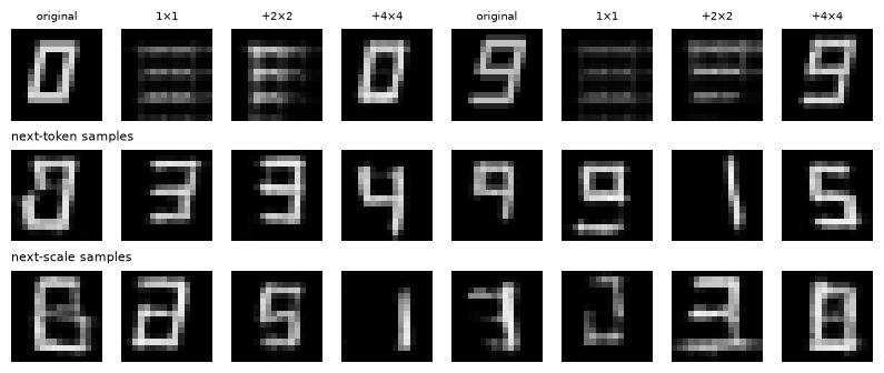
The coarse scales carry little on their own here. The decoder was trained only on the full sum f̂, and with 4×4 as the finest map there is no room for a gradual pyramid. VAR’s ten scales up to 16×16 are a very different regime.
Next-token vs next-scale (VQ with 256 codes, the same 2-layer Transformer, 2000 steps):
| model | tokens / image | sampling steps | time for 2000 samples | test NLL (bits / image) | samples: valid / FID |
|---|---|---|---|---|---|
| next-token (raster) | 16 | 16 | 0.87 s | 54.0 | 0.506 / 27.2 |
| next-scale (VAR) | 21 | 3 | 0.24 s | 88.0 | 0.310 / 37.7 |
Next-scale was 3.6× faster but lost on quality at our scale. Two of Lecture 5’s prices add up:
- Redundant bits. The pyramid describes every image with 21 tokens instead of 16, so the NLL counts redundant bits.
- Independence within a scale. The 16 finest tokens, which here carry almost all the information, are sampled independently given the coarser scales.
We reproduce VAR’s mechanism and its speed, not its quality advantage. That rests on a deep pyramid, much larger models and ImageNet-scale data.
5. TiTok: an image is worth a few tokens (Yu et al. 2024)
5.1 Motivation
Grid tokenizers give every patch its own token, however little the patch contains. Images are highly redundant: neighbouring patches are correlated, backgrounds repeat, and a few global factors (object, pose, style) explain much of the content. TiTok asks: if tokens were not tied to positions, how few would an image need?
5.2 The 1-D tokenizer
- Encoder. A ViT reads the image patches together with K learnable latent tokens. Only the latent tokens’ outputs are kept and quantized — a 1-D sequence with no spatial layout.
- Decoder. Another ViT takes the K quantized tokens plus one learnable mask token per patch position, and each mask token’s output is decoded into its patch.
The paper represents a 256×256 image with as few as 32 tokens (vs 256 or 1024 for 2-D grids). It trains in two stages, first with “proxy codes” from an existing VQGAN, then end to end. A MaskGIT-style generator on these short sequences reaches competitive ImageNet quality with far faster generation.
5.3 Experiment: 1-D tokens on glyphs
Code 04 builds a small version: 2 Transformer layers of width 64 in each of the encoder and decoder, VQ with 256 codes, 1500 steps.
| tokenizer | bits / image | RMSE | valid recon | FID recon |
|---|---|---|---|---|
| 1-D, K = 2 | 16 | 0.088 | 0.822 | 24.7 |
| 1-D, K = 4 | 32 | 0.079 | 0.903 | 14.2 |
| 1-D, K = 8 | 64 | 0.077 | 0.943 | 13.8 |
| grid, 16 tokens × 16 codes | 64 | 0.080 | 0.912 | 11.3 |
| grid, 16 tokens × 256 codes | 128 | 0.052 | 0.978 | 2.1 |
- Very few tokens suffice. Two tokens — 16 bits per image — already reconstruct 82% of glyphs validly. Four tokens (32 bits) match the grid tokenizer with twice the bit budget, and eight beat it in validity. A glyph has only a digit and six style factors; latent tokens that can look anywhere spend their bits on those, not on mostly empty patches.
- The decoder is the limit at the high end. With 128 bits the grid tokenizer is still sharper: our small 1-D decoder, trained briefly, is the limit. With only 1200 steps, K = 8 was even worse than K = 4 — Transformer tokenizers need more training than the convolution-like grid one.
What does each token encode? Mutual information (bits) between each of the four tokens and the true factors:
| factor | token 0 | token 1 | token 2 | token 3 |
|---|---|---|---|---|
| digit (max 3.32) | 2.02 | 1.42 | 1.99 | 1.68 |
| dx (max 2) | 1.40 | 0.67 | 1.37 | 0.33 |
| dy (max 2) | 0.33 | 1.08 | 0.32 | 0.95 |
| slant (max 2) | 1.03 | 0.48 | 1.01 | 0.21 |
| thick / ink (max 2) | 0.27 / 0.24 | 0.42 / 0.28 | 0.27 / 0.22 | 0.49 / 0.27 |
(The estimates are biased upward by up to ~0.3 bit with 256 codes and 2000 images.)
- The tokens specialize without being told. Tokens 0 and 2 encode horizontal position and slant, tokens 1 and 3 vertical position, and every token carries part of the digit.
- Thickness and ink are encoded weakly. They change few pixels, so the reconstruction loss cares little about them.
The tokens are a learned code for the whole image, organized by what reduces the reconstruction error most.
Generation on 1-D tokens (the same small Transformer prior as in §3):
| tokens | sampling steps | valid | FID |
|---|---|---|---|
| 1-D, K = 4 | 4 | 0.856 | 20.3 |
| 1-D, K = 8 | 8 | 0.869 | 22.5 |
| grid, 16 × 256 codes (§3.2) | 16 | 0.506 | 27.2 |
A compact tokenizer helps generation twice:
- the sequences are shorter;
- they are less redundant — the prior no longer has to learn that 12 of 16 patches are empty background, in a hundred consistent ways.
The samples come close to the tokenizer’s own ceiling. This is TiTok’s argument, and the clearest result of this lecture’s experiments.
6. The big picture
6.1 What a tokenizer decides
| decision | options in this lecture | effect on the prior |
|---|---|---|
| unit | pixels (iGPT) / patches (DALL·E, grid) / scales (VAR) / latent tokens (TiTok) | sequence length and redundancy |
| quantizer | VQ / FSQ / LFQ | codebook usage, maximum vocabulary |
| vocabulary | 16 … 2^18 | ceiling vs difficulty (§3.2) |
| order | raster / coarse-to-fine / none (1-D) | number of steps, what each step conditions on |
6.2 The five components of the two-stage model
| component | tokenizer | prior |
|---|---|---|
| formulation | lossy compression to discrete codes | chain rule over tokens (by token, by scale, or masked) |
| representation | CNN / ViT encoder and decoder + quantizer | causal or block-causal Transformer |
| objective | reconstruction (+ perceptual, adversarial in practice: VQ-GAN, Lecture 9) + quantizer losses | cross-entropy (exact likelihood of tokens) |
| optimization | straight-through gradients, restarts, entropy losses | teacher forcing |
| inference | encode / decode | sequential sampling (fewer steps with scales or short 1-D sequences) |
Note that likelihoods are exact only for tokens. The pipeline as a whole is not a likelihood model of pixels, because the tokenizer is lossy.
6.3 Where this goes
- Lecture 8 asks whether tokens need to be discrete at all. MAR keeps continuous tokens and models each one’s conditional with a small diffusion model; Transfusion and Show-o put text tokens and image tokens in one Transformer.
- Lecture 9 adds the adversarial and perceptual losses that make real tokenizers sharp (VQ-GAN). Every production tokenizer uses them; ours used plain squared error.
- Latent diffusion (Lecture 13) uses the same idea with continuous latents: a tokenizer-like autoencoder plus a generator in its latent space.
7. Summary
- Two stages. Modern autoregressive image generation is tokenizer + prior. The tokenizer sets the ceiling (decoding real tokens) and the prior adds its own errors (decoding sampled tokens). A small Transformer prior turned Lecture 3’s tokenizer from FID 166 (bigram) into FID 27.
- Quantizers. VQ learns a codebook and needs restarts against dead codes (8% usage without them at K = 1024). FSQ rounds a few scalars to a fixed grid. LFQ takes signs and needs an entropy loss (4 of 1024 codes without it; the paper’s weight was too small at our scale). VQ with restarts reconstructed best here.
- The vocabulary is a trade-off. Bigger codebooks raised the ceiling and lowered sample quality from the same prior (valid 0.65 → 0.33 from K = 16 to 1024), as MAGVIT-v2 reports for VQ.
- VAR predicts whole scales coarse to fine with a block-causal Transformer: few steps and no raster asymmetry. At our scale it was 3.6× faster but worse, because a three-scale pyramid adds redundant tokens and samples its finest map independently.
- TiTok’s 1-D latent tokens describe an image with far fewer tokens: 4 tokens (32 bits) matched a 64-bit grid tokenizer. The tokens specialized (position, slant, digit) on their own, and a prior on them produced the best samples of the lecture (valid 0.86–0.87).
8. Common pitfalls
- “A bigger codebook is always better.” It improves reconstruction, not necessarily generation (§3.2).
- “Codebook size = number of codes in use.” Check usage and perplexity; VQ without restarts used 8% of its codes (§2.2).
- “LFQ / FSQ need no tuning.” FSQ has no auxiliary loss, but LFQ’s entropy weight decided between 4 and 720 codes in use (§2.2).
- “The tokenizer’s reconstruction quality is the generator’s quality.” Decoded real tokens are an upper bound; decoded sampled tokens can be far worse (§1.3, §3.2).
- “Next-scale prediction is free speed.” Predicting a whole scale at once ignores dependencies within it; small pyramids add redundant tokens (§4.4).
- “Tokens must correspond to image patches.” 1-D latent tokens need not, and can be much more compact (§5).
- “The two-stage model has an exact image likelihood.” Only the tokens’ likelihood is exact; the tokenizer is lossy (§6.2).
9. Exercises
Exercise 1 (bits). A grid tokenizer turns a 256×256 image into 16×16 tokens from a codebook of 1024. (a) How many bits can the token sequence describe? (b) Compare with the raw image (8 bits per sub-pixel). (c) What compression ratio is that, and why can it still give good-looking reconstructions?
Answer
(a) 256 · log₂1024 = 2560 bits.
(b) The raw image has 256·256·3·8 = 1,572,864 bits.
(c) About 600× compression. Natural images are highly redundant, and perceptually unimportant details (exact noise, small texture variations) can be dropped. Real tokenizers add perceptual and adversarial losses so that the decoder invents plausible high-frequency detail rather than reproducing it.
Exercise 2 (FSQ). For levels (8, 5, 5, 5): (a) how many codes? (b) write the index of a code with levels (q₁, q₂, q₃, q₄) as a mixed-radix number; (c) why can no FSQ code be “dead” in the VQ sense, and what can still go wrong?
Answer
(a) 8·5·5·5 = 1000.
(b) idx = q₁ + 8q₂ + 40q₃ + 200q₄, with q_i ∈ {0, …, L_i − 1}.
(c) Codes are not parameters, so there is nothing that fails to receive a gradient. But the encoder may still never produce some combinations, so codes can go unused (code 01: 697 of 1024 used, perplexity 230). Also, the grid’s resolution per dimension is fixed: rare but important variations may fall between grid points.
Exercise 3 (LFQ’s entropy loss). Show that E[H(p(·|z))] − H(E[p(·|z)]) = −I(code; z) under the soft assignment, i.e. minimizing it maximizes the mutual information between the input and the code. What do its two terms do separately?
Answer
For a joint distribution p(z) p(c | z), the mutual information is I(c; z) = H(c) − H(c | z), with H(c) = H(E_z[p(c | z)]) and H(c | z) = E_z[H(p(· | z))]. So the loss equals H(c | z) − H(c) = −I(c; z).
- Minimizing H(c | z) makes every z commit to one code.
- Maximizing H(c) spreads the codes evenly over the data.
Together they maximize how much the code says about the input — the information-theoretic ideal of a tokenizer with a fixed number of bits.
Exercise 4 (the vocabulary trade-off). A prior with test NLL N bits per image samples token sequences. (a) Why can a larger vocabulary increase N even though it describes images better? (b) Code 02 measured N = 23.8, 54.0 and 75.6 bits for K = 16, 256, 1024. If the prior were perfect, what would these numbers converge to as data → ∞?
Answer
(a) N is the entropy of the token distribution under the prior plus the prior’s KL to the truth. A larger vocabulary makes token sequences carry more information about each image (finer distinctions), so the true entropy of the tokens grows. The prior must also learn a larger distribution from the same data, so its KL grows too.
(b) To the true entropy of the token sequences under the data distribution, H(tokens) ≤ 16·log₂K. For a deterministic tokenizer it is the entropy of the quantized description of a random glyph: larger for larger K, bounded by the information in a glyph (a digit plus continuous style, quantized finely enough).
Exercise 5 (next-scale independence). In VAR, the tokens of scale k are sampled independently given the coarser scales. Using Lecture 5 §2.3, write the extra cost (in bits) of this choice compared with sampling scale k’s tokens autoregressively. When is it small?
Answer
The extra cost is the conditional total correlation of scale k’s tokens given the coarser scales: Σ_j H(r_{k,j} | r_{<k}) − H(r_k | r_{<k}).
It is small when the coarser scales already determine most of the dependence between scale k’s tokens — e.g. when a fine map mostly adds local, nearly independent detail to a good coarse structure. That is the regime of a deep pyramid, and not of our three-scale toy, where the finest map carries almost everything.
Exercise 6 (block-causal masks). Write the 5×5 attention mask (True = blocked) for scales 1×1 and 2×2 in VAR’s order. Why may tokens of the same scale attend to each other, given that their own tokens are predicted from these positions?
Answer
Positions: [s1], [s2a, s2b, s2c, s2d]. Row s1 blocks the four s2 columns; rows s2* block nothing (they may attend to s1 and to each other).
This is safe because the inputs at scale-2 positions are built only from scale 1 (the upsampled f̂ of coarser scales), never from scale-2 tokens. Attending to each other shares information about the coarse context, not about the answers. The same holds in code 03, where changing scale 2’s tokens left scale 2’s predictions unchanged.
Exercise 7 (1-D vs 2-D). Why can a 1-D tokenizer use far fewer tokens than a grid tokenizer for the same reconstruction quality? Give one reason why grid tokens might still be preferable for some tasks.
Answer
Why fewer tokens. Grid tokens must each describe their own patch, so redundancy between patches (empty background, repeated structure, global factors shared by all patches) is paid for many times. Latent tokens can describe global factors once and spend their bits where the information is.
Why grid tokens can still be preferable. They keep spatial correspondence. Local editing, inpainting, spatial conditioning (layouts, masks), and models that rely on locality (convolutions, spatial attention patterns) work naturally on grids. With 1-D tokens, changing one region of the image can require changing all tokens.
Exercise 8 (hands-on).
(a) In 02_token_ar.py, double the prior’s width and depth for K = 1024. How much of the gap to K = 16 closes?
(b) In 03_next_scale.py, add a fourth scale between 2×2 and 4×4 (3×3). Does the pyramid become more gradual?
(c) In 04_one_d_tokens.py, replace VQ with FSQ (8, 5, 5, 5). Do the tokens still specialize?
Answer (sketch)
(a) A larger prior should help the large vocabulary more than the small one (it has more to learn). Expect part of the gap to close, but with 20,000 images data become the limit.
(b) A 3×3 scale adds 9 tokens. It makes the coarse part of the pyramid more informative, but also more redundant. Watch both the partial-decode recognizability and the NLL.
(c) Probably yes. Specialization comes from the encoder learning where to put information, not from the quantizer type. FSQ’s fixed grid may encode continuous factors (position, slant) more smoothly.
10. Further reading
The required and optional papers
- L. Yu et al., Language Model Beats Diffusion — Tokenizer is Key to Visual Generation, ICLR 2024.
- K. Tian et al., Visual Autoregressive Modeling: Scalable Image Generation via Next-Scale Prediction, NeurIPS 2024.
- Q. Yu et al., An Image is Worth 32 Tokens for Reconstruction and Generation, 2024.
- M. Chen et al., Generative Pretraining from Pixels, ICML 2020.
- A. Ramesh et al., Zero-Shot Text-to-Image Generation, ICML 2021.
- F. Mentzer, D. Minnen, E. Agustsson, M. Tschannen, Finite Scalar Quantization: VQ-VAE Made Simple, ICLR 2024.
Background
- A. van den Oord, O. Vinyals, K. Kavukcuoglu, Neural Discrete Representation Learning (VQ-VAE), NeurIPS 2017; A. Razavi et al., VQ-VAE-2, NeurIPS 2019.
- P. Esser, R. Rombach, B. Ommer, Taming Transformers for High-Resolution Image Synthesis (VQ-GAN), CVPR 2021 (Lecture 9).
- H. Chang et al., MaskGIT: Masked Generative Image Transformer, CVPR 2022 (the masked generator used by MAGVIT-v2 and TiTok).
- D. Lee et al., Autoregressive Image Generation using Residual Quantization (RQ-VAE), CVPR 2022: residual quantization at one scale, a precursor of VAR’s.
- J. Yu et al., Scaling Autoregressive Models for Content-Rich Text-to-Image Generation (Parti), 2022.
Related notes in this course
- Lecture 3 §7 (VQ-VAE, dead codes, “a tokenizer is not a generator”).
- Lecture 5 §2.3 (the cost of predicting blocks independently), §5 (causal masks).
11. Next lecture
Lecture 8: Autoregression meets diffusion (reading session · 10/01).
Everything in this lecture relied on discrete tokens, because a softmax is the easiest way to represent a conditional distribution. But quantization loses information, and tokenizers are hard to train. Lecture 8’s papers question this:
- MAR keeps continuous tokens and represents each token’s conditional distribution with a small diffusion model (the “diffusion loss”), generating in a random order with several tokens per step;
- Transfusion trains one Transformer with next-token prediction on text and diffusion on images;
- Show-o unifies autoregressive text and discrete masked image modeling for understanding and generation.
We will see why a regression head fails for continuous tokens (Lecture 1’s ghosts again) and how a small diffusion head fixes it.