Maps to: MIT 6.S978 Deep Generative Models (Fall 2024), Reading · Tue 09/17/2024 · Normalizing Flows (student paper session). Required papers:
- D. Rezende & S. Mohamed, Variational Inference with Normalizing Flows, ICML 2015;
- D. P. Kingma & P. Dhariwal, Glow: Generative Flow with Invertible 1×1 Convolutions, NeurIPS 2018;
- J. Behrmann, W. Grathwohl, R. T. Q. Chen, D. Duvenaud & J.-H. Jacobsen, Invertible Residual Networks, ICML 2019.
Optional: Lilian Weng, Flow-based Deep Generative Models (blog, 2018). Basis: This session consisted of student presentations, with no published slides. These notes are organized around the three papers:
- the question they share — “can a generator be invertible, so that its density is exact?”;
- the background they need (change of variables, coupling layers from NICE / RealNVP);
- each paper’s motivation, method, results and limitations.
Numbers taken from the papers are labelled “the paper reports”. All experiments were designed for these notes and run on a CPU, on 2-D toy densities with known formulas and on GlyphWorld. Several outcomes contradicted my plan; they are reported as they came out, and the code README lists them. Code:
code/lecture04/— 6 scripts + the shared moduleflow_tools.py. Each script runs in 30–80 s. Reading time: 4–5 hours including running the code.
0. How to read this lecture
0.1 Where we are
Lecture 3 built a generator from a simple latent z and a neural decoder, and paid twice for it:
- the likelihood p_θ(x) became an integral nobody can compute;
- the posterior p_θ(z | x) lost its formula.
The VAE gave up on both and optimized a lower bound, the ELBO. The gap between the bound and the truth is KL(q ‖ posterior), and Lecture 3 measured it: 0.737 nat for a Gaussian q facing a bimodal posterior, even in a one-dimensional toy.
Normalizing flows take the opposite route: make the generator invertible. If x = f(z) and z = f⁻¹(x) are both computable, and f is built from pieces whose Jacobian determinants are cheap, then nothing is hidden. Every x has exactly one z, and the density of x follows from the change-of-variables formula exactly. There is no integral, no posterior and no bound.
The three papers use this idea in three ways:
| Paper | What the flow is for | How the determinant is made cheap |
|---|---|---|
| Rezende & Mohamed 2015 | a richer approximate posterior q(z | x) inside a VAE | each layer is identity + rank one → matrix determinant lemma |
| Kingma & Dhariwal 2018 (Glow) | an exact-likelihood image model p(x) | triangular Jacobians (coupling layers) + an LU-factorized 1×1 convolution |
| Behrmann et al. 2019 (i-ResNet) | a standard ResNet that is also a density model | no special structure; a power series for log det, estimated stochastically |
0.2 Learning goals
- Write the change-of-variables formula for a composition of maps, and say which direction (latent → data or data → latent) must be cheap for variational inference and for density estimation.
- Name the three structural costs of flows: the determinant, guaranteed invertibility, and preserved dimension and topology. Explain why a continuous bijection cannot map a Gaussian onto disconnected islands, and what “bridges” are.
- Derive the log-det of planar and radial flows, and the invertibility condition wᵀu ≥ −1. Explain how flows shrink the approximation gap of a VAE, and why reverse KL and optimization limit what they achieve in practice.
- Explain affine coupling layers: why the Jacobian is triangular, why the inverse is free, and why the inner network can be anything.
- Describe Glow’s step of flow (ActNorm → invertible 1×1 convolution → affine coupling) and its multi-scale architecture. Compute bits/dim with uniform dequantization. Explain temperature sampling and latent-space manipulation.
- Prove that y = x + g(x) is invertible when Lip(g) < 1. Invert it by fixed-point iteration. Derive the power series for log det(I + J_g), and explain Hutchinson’s estimator and the truncation bias.
- Place flows among the model families: what they buy (exact likelihood, exact inference), what they cost (architecture constraints, sample quality), and where their ideas live on (IAF in Lecture 6, the probability-flow ODE in Lecture 12, flow matching in Lecture 16).
0.3 Map
| Section | Content | Code |
|---|---|---|
| §1 | Change of variables; two directions; the three costs; bridges | — |
| §2 | Rezende & Mohamed: planar and radial flows for variational inference | 01_planar_radial_vi.py, 02_flow_posterior.py |
| §3 | Coupling layers (NICE, RealNVP): the workhorse | 03_coupling_flows.py |
| §4 | Glow: ActNorm, 1×1 convolutions, multi-scale, temperature | 04_glow_components.py, 05_glow_glyphs.py |
| §5 | Invertible residual networks | 06_iresnet.py |
| §6 | The big picture | — |
0.4 Notation and the two directions
| Symbol | Meaning |
|---|---|
| x ∈ ℝ^D | data; z ∈ ℝ^D the latent — the same dimension |
| p_Z | base density, N(0, I) unless stated |
| f | an invertible map; J_f(·) its Jacobian matrix; |det J_f| its absolute determinant |
| f = f_K ∘ … ∘ f_1 | a flow: a composition of K invertible layers |
| T | sampling temperature: z ~ N(0, T² I) |
Papers disagree on which way f points:
- Rezende & Mohamed write the generative direction z₀ → z₁ → … → z_K.
- Glow and i-ResNet write f as data → latent (x ↦ z), because density evaluation is what training needs.
These notes say each time which direction is meant. The code follows the same split: PlanarFlow.forward is generative, Coupling2D.forward is data → latent.
1. Change of variables · What makes a flow
1.1 The formula, and why it holds
Push a random variable z with density p_Z through an invertible, differentiable map x = g(z). In 1-D, probability mass is conserved: the mass in a tiny interval dz around z equals the mass in the interval dx around x = g(z). So p_X(x)|dx| = p_Z(z)|dz|, and
Where g stretches space (|g′| > 1), the same mass is spread over more room and the density drops. Where it compresses, the density rises.
In D dimensions a tiny box becomes a tiny parallelepiped whose volume is scaled by |det J|. With f = g⁻¹ the data → latent map:
P1 §6 checked this numerically in 1-D and 2-D. The whole art of normalizing flows is to make this formula cheap and guaranteed for maps flexible enough to turn a Gaussian into images.
1.2 Compositions: log-dets add
The determinant of a product of matrices is the product of determinants. By the chain rule, the Jacobian of f = f_K ∘ … ∘ f_1 is the product of the layers’ Jacobians, so
Each layer can be simple; the stack becomes expressive. This is where the name comes from: a simple density “flows” through the layers and is “normalized” back into a valid density at every step.
1.3 Two directions, two jobs
| Job | What you must compute | Which direction must be cheap |
|---|---|---|
| Density estimation (train on data by maximum likelihood) | log p(x) at data points | data → latent, plus its log-det |
| Sampling | x = g(z) for fresh z | latent → data |
| Variational inference (a flexible q) | samples of q and log q at those same samples | latent → data only, plus its log-det along the way |
The last row is why Rezende & Mohamed can use layers with no closed-form inverse. VI never asks “what is q at this given point?”, only “give me a sample and its density”. Glow needs both directions to be cheap, so its layers must be invertible in closed form. i-ResNet needs data → latent in closed form and pays an iterative solve for sampling. Lecture 6 meets the same trade-off in its sharpest form: MAF (fast density, slow sampling) vs IAF (fast sampling, slow density).
1.4 The three costs of invertibility
-
The determinant. A generic D×D determinant costs O(D³). For a 64×64×3 image, D ≈ 12,000, and the cost recurs at every layer and every training step. Every flow is a way to make it cheap:
trick layers rank-one updates planar triangular Jacobians coupling, autoregressive factorized matrices LU stochastic estimates i-ResNet -
Invertibility must be guaranteed by construction. A layer that is invertible “for most parameter values” is not enough: gradient descent will find the others. Each paper has a constraint or parameterization that makes invertibility automatic: û for planar flows, exp(s) > 0 for couplings, Lip(g) < 1 for i-ResNets.
-
Dimension and topology are preserved.
- The latent has as many dimensions as the data: no compression, unlike a VAE.
- A continuous bijection maps a connected set onto a connected set. A Gaussian has one connected support, so a flow can never put zero mass between two modes. It can only make the connecting bridges thin, at the price of enormous stretching.
§3.4 measures the bridges, and §4.5 shows that they also cost sample quality on images.
Intuition. A flow is a perfectly reversible rubber sheet. You may stretch, squeeze, bend and fold it smoothly, but you may never cut it or glue it. Every density a flow can express is a Gaussian on such a deformed sheet.
2. Rezende & Mohamed (2015) · Flows for variational inference
2.1 Motivation: the posterior family is the bottleneck
Variational inference trades exactness for tractability. The ELBO gap is KL(q ‖ p(z | x)), and with a diagonal Gaussian q it can never vanish unless the true posterior happens to be a diagonal Gaussian. Lecture 3 showed what that costs: a bimodal posterior with a symmetric shape left a gap of 0.737 nat for the best Gaussian. Worse, Lecture 3 §3 showed that a model trained with the ELBO bends itself toward posteriors that are easy to approximate — the bias of the approximation leaks into the model.
The paper’s argument: we want a family of q’s that is
- rich, ideally able to approach the true posterior arbitrarily well;
- cheap to sample;
- cheap to evaluate at its own samples (the ELBO needs log q(z));
- amortizable: an encoder network can output its parameters for each x, as in a VAE.
Their answer: start from a diagonal Gaussian z₀ ~ q₀(z₀ | x) and apply K invertible maps, z_K = f_K ∘ … ∘ f_1(z₀). Then
The ELBO becomes the “flow-based free energy” (the paper’s eq. 15):
Every term is an average over samples z₀ ~ q₀, so the reparameterization trick (Lecture 3 §4) applies unchanged.
2.2 Planar and radial flows
The paper proposes two families with O(D) log-dets.
Planar flow.
It moves every point along the direction u, by an amount that depends on which side of the hyperplane wᵀz + b = 0 the point lies. In the paper’s words, it contracts or expands the density perpendicular to that hyperplane. The Jacobian is I + u ψ(z)ᵀ with ψ(z) = h′(wᵀz + b) w, an identity plus rank one. The matrix determinant lemma gives
O(D) instead of O(D³).
Radial flow.
It pulls points toward a reference point z₀ (β < 0) or pushes them away (β > 0), strongly nearby and weakly far away. Its determinant is
again O(D).
Invertibility. Neither layer is automatically invertible. For the planar flow with h = tanh, f is invertible iff wᵀu ≥ −1 (exercise 1). The paper’s appendix enforces this with a reparameterization:
which guarantees wᵀû > −1 for any raw u. For the radial flow the condition is β ≥ −α.
Code 01, part 1 checks the mechanics:
- The O(D) formula matches a full autograd Jacobian to ≤ 1.4e−6 for D = 2, 10, 50.
- In 1-D with w = 1:
- raw u = −2 gives min f′ = −1.0, and the layer folds the line onto itself;
- the corrected û = −0.873 gives min f′ = +0.127, and the layer stays invertible;
- for positive w·u the correction barely changes u.
The paper also discusses infinitesimal flows: Langevin dynamics and Hamiltonian flows, whose densities evolve by known PDEs, so that in a limit the family can represent the true posterior exactly. These are the ancestors of the continuous-time flows of §6.3. The paper’s experiments use finite flows.
2.3 What the paper reports
- 2-D test densities (the paper’s Figure 3). Four unnormalized densities p(z) ∝ exp(−U(z)) — a ring split into two lobes, and three variants of a sine-shaped band — are approximated with planar and radial flows of length K = 2, 8, 32. Longer flows match the targets visibly better, and planar flows do better than radial ones.
- MNIST. A deep latent Gaussian model (a VAE) with a diagonal-Gaussian posterior reaches a bound of −log p(x) ≤ 89.9 nats. Adding planar flows of length 10, 20, 40 and 80 improves the bound steadily, to about 85.1 nats at K = 80. Volume-preserving NICE-style flows of the same length improve it less. The CIFAR-10 experiments show the same ordering.
2.4 Our experiments
The four energies (code 01, part 2). One complication: as written, U2–U4 only constrain z₂ relative to a function of z₁, so exp(−U) has infinite mass. A q that keeps spreading along the band lowers the objective forever, and my first KL estimates came out negative. We add a soft wall at |z₁| = 4, the edge of the paper’s plots.
We fit q_K by minimizing E_q[log q + βU] with β annealed from 0.01 to 1 (as in the paper), for 2000 steps each with one fixed seed. log Z comes from a fine grid, so KL(q ‖ p) is exact up to Monte Carlo error:
| target | planar K=2 | planar K=8 | planar K=32 | radial K=8 | radial K=32 |
|---|---|---|---|---|---|
| U1 (two-lobed ring) | 0.825 | 0.106 | 0.030 | 0.206 | 0.118 |
| U2 (sine band) | 0.817 | 0.291 | 0.446 | 0.787 | 0.484 |
| U3 (splitting bands) | 1.017 | 0.417 | 0.194 | 0.751 | 0.463 |
| U4 (band + step) | 1.091 | 0.301 | 0.297 | 0.815 | 0.546 |
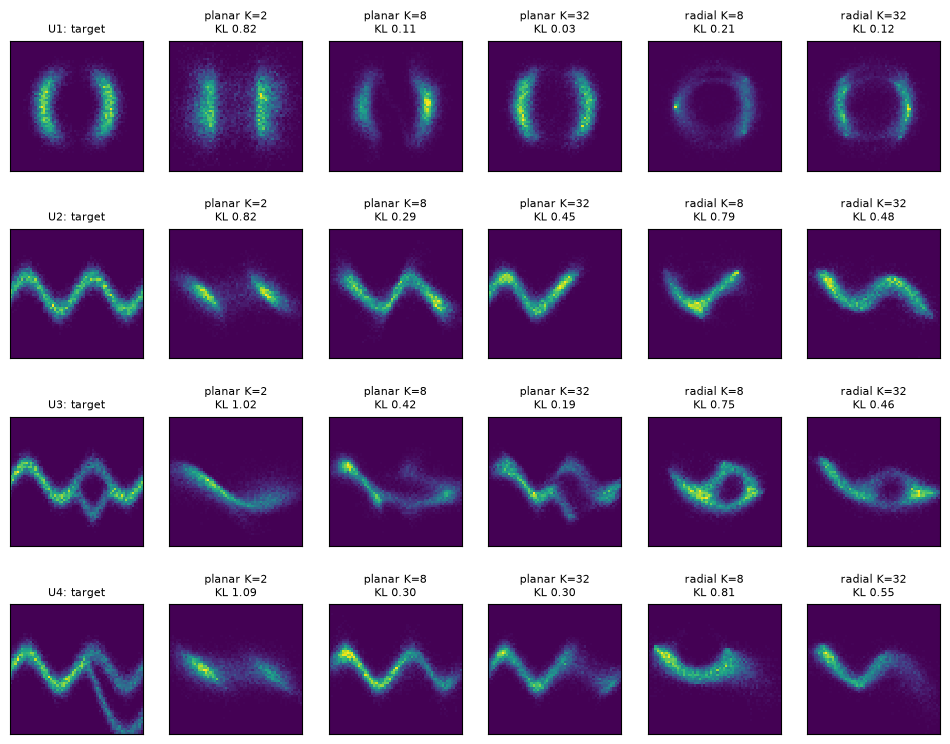
- Planar beats radial at equal K on every target, as in the paper. These targets are bands and rings, easier to build from hyperplane-wise stretches than from pulls around points.
- More layers usually help (U1: 0.825 → 0.106 → 0.030), but not always. On U2, 32 planar layers ended worse than 8 (0.446 vs 0.291). That q put only 0.244 of its mass on the right half of the band, where the target has 0.499: it modeled the left half well and dropped the rest. A two-seed check gave 0.445 and 0.096 for this setting, so it is an optimization outcome, not a capacity limit.
- Reverse KL charges little for missing parts of p (Lecture 1 §5.3). That is how a q missing half the band can still have a moderate KL. It is also why on U4 every q puts too little mass on the second band (0.36–0.42 vs 0.487).
Closing Lecture 3’s gap (code 02). The toy of Lecture 3 has a 1-D latent and an exactly computable posterior:
Its posterior is unimodal (case A), bimodal and lopsided (B), or bimodal and symmetric (C). We put K one-dimensional planar flows on a learnable Gaussian, maximize the ELBO with annealing, and report the gap log p(x) − ELBO for three seeds:
| K | A (unimodal) | B (bimodal, lopsided) | C (bimodal, symmetric) |
|---|---|---|---|
| 0 (Gaussian) | 0.0037 / 0.0037 / 0.0037 | 0.1748 / 0.1749 / 0.1749 | 1.6285 / 1.6285 / 1.6286 |
| 2 | 0.0008 / 0.0040 / 0.0036 | 0.1443 / 0.1445 / 0.1442 | 0.6921 / 1.6368 / 1.6377 |
| 4 | 0.0023 / 0.0025 / 0.0035 | 0.1346 / 0.0699 / 0.1378 | 0.0722 / 0.0806 / 0.0983 |
| 8 | 0.0005 / 11.9199 / 0.0010 | 0.0025 / 0.1537 / 0.0111 | 0.0012 / 0.0749 / 0.0022 |
(Lecture 3’s best Gaussian: 0.0034, 0.174, 0.737.)
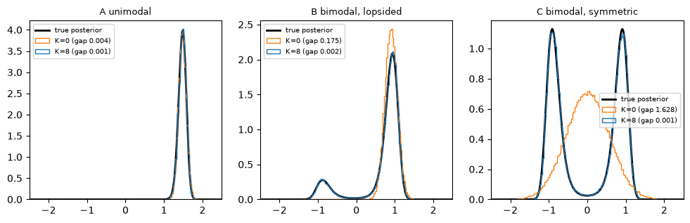
- When it works, it works. Two of three seeds with K = 8 reach the true posterior within about 0.01 nat in every case; on the bimodal cases the gap shrinks 15 to 600 fold. In 1-D, a planar layer with large u·w stretches the middle of the line and thins the density there: that is how one bump becomes two.
- The failures are instructive.
- Case A, seed 1, settles on the mirror mode z ≈ −1.4, although x₂ = 0.75 says z is positive. The 11.9 nats are the likelihood penalty of the wrong sign.
- Case B, seed 1, covers only the right mode (mass on z > 0 is 1.000; truth 0.867).
- Annealing flattens the target early, so both signs look equally plausible, and q can commit to the wrong one before β reaches 1.
- Without annealing (case C, β = 1 from the start), flows with K ≥ 4 lock onto one mode, with gaps of 0.67–0.74. Dropping one of two equal modes costs about log 2 = 0.693: a perfect fit to one half of a symmetric posterior is off by exactly a factor 2 in density. The gap is slightly below log 2 here because the modes overlap near z = 0.
- A Gaussian started at z = 0 stays symmetric, straddling both modes (gap 1.63), annealed or not. It is worse than Lecture 3’s Gaussian placed on one mode.
Lesson. A richer q-family removes the capacity limit of variational inference, not its optimization problem. The reverse KL in the ELBO still prefers to sit on one mode, and getting a flexible q to cover several modes needs help (annealing, several restarts) — and still fails sometimes.
2.5 Where this went
Planar flows turned out to be too weak for high-dimensional posteriors: each layer changes the density along a single direction. The idea of “a flow inside the VAE” survived in stronger forms. Inverse autoregressive flows (IAF, Kingma et al. 2016, Lecture 6) use autoregressive layers with triangular Jacobians. Volume-preserving and Sylvester flows came later. The density-estimation use of flows took off with coupling layers, which come next.
3. Coupling layers · The workhorse
Glow builds on two earlier papers by Dinh et al.: NICE (2014) and RealNVP (2017). Their key idea is needed to read Glow.
3.1 The affine coupling layer
Split the input into two parts x = (x_a, x_b). Keep x_a, and use it to compute a scale and a shift for x_b (data → latent direction):
Three properties follow immediately:
-
Triangular Jacobian. ∂y_a/∂x_b = 0, so the Jacobian is block triangular. Its diagonal blocks are I and diag(exp s(x_a)), so
The log-det is a sum over one network output.
-
Free inverse. Since y_a = x_a, the inverse is x_b = (y_b − t(y_a)) ⊙ exp(−s(y_a)). There is no iteration and no matrix inverse.
-
Any network for s and t. They are never inverted and never differentiated for the determinant, so they can be arbitrarily deep, nonlinear and non-invertible.
NICE is the special case s ≡ 0 (additive coupling, log-det 0, “volume preserving”). RealNVP adds the scale.
One layer leaves x_a untouched, so layers alternate which part they keep. In images, RealNVP alternates checkerboard and channel-wise splits and uses a squeeze operation that turns each 2×2×C block into 1×1×4C. That trades resolution for channels, so that later layers see more context. It also uses a multi-scale architecture that factors out half of the dimensions at each level (Glow keeps it; §4.3).
Code 03, part 1 checks one layer:
- the round-trip error is 9.5e−7;
- the Jacobian at a test point is [[1.000, 0.000], [−0.995, 3.711]]: triangular, with the exact zero;
- the formula log-det matches autograd to 9.5e−7.
3.2 Experiment: depth on 2-D targets with exact densities
Code 03 trains RealNVP by maximum likelihood on fresh samples from two targets whose densities we know, so KL(p ‖ model) = NLL − H(p) is exact:
- ring: 8 Gaussians (std 0.25) on a circle of radius 2;
- checkerboard: uniform on 8 black squares, with sharp edges and empty squares.
| target | couplings | parameters | KL | low-density / off the squares | mode share (ideal 0.125) |
|---|---|---|---|---|---|
| ring | 2 | 38,600 | 0.675 | 0.270 | 0.092–0.145 |
| ring | 4 | 77,200 | 0.198 | 0.055 | 0.112–0.138 |
| ring | 12 | 231,600 | 0.095 | 0.019 (true: 0.010) | 0.119–0.137 |
| checkerboard | 12 | 231,600 | 0.271 | 17.6% off the squares | — |
(“Low-density” is the fraction of samples where the true density is below its own 1st percentile; real data give 0.010.)
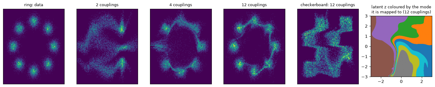
- Depth. Two couplings can bend the Gaussian only twice; twelve separate all 8 modes.
- Exactness. Every NLL in the table is exact, from one forward pass — no bound, no sampling. This is what flows buy.
- Cost. It took more than I planned: my first design (8 couplings, small MLPs, 3000 steps) stopped at KL 0.24 on the ring and 0.41 on the checkerboard. Flows with simple layers are slow learners, and even the final checkerboard model smears 17.6% of its samples across the sharp edges.
3.3 Bridges: the price of continuity
A flow cannot tear the plane, so the boundaries between the 8 “mode regions” in latent space must map somewhere in data space: onto bridges between modes. Code 03, part 3 looks at where the bridge samples come from:
| samples | fraction | a 0.05-step in z changes the mode | median |z| |
|---|---|---|---|
| bridge (low density) | 0.018 | 0.246 | 2.80 |
| all others | 0.982 | 0.086 | 1.17 |
Bridge samples sit near region boundaries, as expected. A tiny latent step crosses into another mode three times as often as for other samples.
I expected them to come from typical latents. They do not: their median |z| is 2.8, deep in the tail of the base. The last panel of the figure shows why. The learned mode regions are not pie slices around z = 0 but bent bands, whose boundaries crowd together far from the origin. The flow has learned to put its unavoidable cuts where the Gaussian has little mass. It cannot remove the bridges, but it can make them cheap.
3.4 Temperature
Sampling with z ~ N(0, T² I), T < 1, concentrates samples near the center of the base:
| T | low-density | mean distance to nearest center (std; data 1.25) | mode share min–max | entropy of mode shares (bits; ideal 3) |
|---|---|---|---|---|
| 1.0 | 0.020 | 1.42 | 0.117–0.134 | 2.999 |
| 0.8 | 0.007 | 1.29 | 0.088–0.154 | 2.977 |
| 0.6 | 0.004 | 1.22 | 0.045–0.209 | 2.843 |
| 0.4 | 0.004 | 1.18 | 0.008–0.317 | 2.374 |
Because the bridge mass comes from large |z|, a mild temperature removes most of it: at T = 0.8 the low-density share is below that of real data. The price is balance between modes. The center of the base maps to some modes more than others, and at T = 0.4 one mode gets 0.8% of the samples and another 32%. Statistically, T < 1 is a different distribution: it trades coverage for typicality. Glow uses it for exactly that trade.
4. Glow (Kingma & Dhariwal 2018)
4.1 Motivation
By 2018 GANs produced the best-looking images, but flows had properties GANs lack. The paper lists them:
- exact latent-variable inference (every image has exactly one z, computed by one pass);
- exact log-likelihood evaluation (comparable across models, usable for compression or anomaly detection);
- efficient inference and synthesis, both parallel — unlike autoregressive models, which sample pixel by pixel;
- a useful latent space for downstream tasks and manipulation;
- memory savings: activations can be recomputed from the output by inverting each layer, instead of being stored for backpropagation.
The question was whether a flow could produce sharp, large images. Glow’s contributions are a simpler and stronger step of flow, and a demonstration at 256×256 on faces.
4.2 One step of flow: three layers
Each step applies three invertible layers to a tensor of shape H × W × C (data → latent direction):
| Layer | Forward | Inverse | log|det| |
|---|---|---|---|
| ActNorm | y = s ⊙ (x + b), per channel | x = y / s − b | H·W·Σ_c log|s_c| |
| Invertible 1×1 conv | y_{ij} = W x_{ij} at every pixel | x_{ij} = W⁻¹ y_{ij} | H·W·log|det W| |
| Affine coupling | x_a, x_b = split(x); (log s, t) = NN(x_a); y_b = s ⊙ x_b + t | x_b = (y_b − t)/s | Σ log|s| |
Notes on each:
-
ActNorm replaces RealNVP’s BatchNorm. It is a per-channel affine map whose parameters are initialized from the first minibatch, so that that batch comes out with zero mean and unit variance; after that they are ordinary parameters. Glow trained with tiny per-GPU batches, where batch statistics are noisy. ActNorm is exactly invertible and independent of the batch.
-
Invertible 1×1 convolution generalizes RealNVP’s fixed channel permutations: a permutation is a special rotation, and W can learn any mixing. Initialized as a random rotation, |det| = 1. Computing log|det W| costs O(C³); the LU parameterization makes it O(C):
with P a fixed permutation, L unit lower-triangular, and U strictly upper-triangular.
-
Affine coupling, as in §3, with two details:
- the last layer of NN is zero-initialized, so every coupling starts as the identity (a deep flow at initialization is then just the identity, which trains stably);
- the scale is computed as s = sigmoid(raw + 2) in the official code.
Code 04 checks the components:
- ActNorm. After initialization, the first batch has per-channel mean 0.00 and std 1.00 exactly; a new batch comes out at about −0.02 and 0.98–0.99. The log-det formula matches autograd (−6.4183).
- LU 1×1 convolution. Σ log|s| equals slogdet(W) to four decimals for C = 4 … 512. At C = 512, slogdet takes about 490 µs per call and the sum 1 µs.
- Conditioning. The inverse round-trip error grows with the condition number of W: 2.7e−7 at cond 2, 1.6e−3 at cond 890. Invertible is not the same as well-conditioned.
4.3 The multi-scale architecture, and bits/dim
Glow keeps RealNVP’s multi-scale design. Each level consists of:
- a squeeze (H × W × C → H/2 × W/2 × 4C);
- K steps of flow;
- a split: half of the channels are declared final latents and modeled by a Gaussian whose mean and scale are predicted from the other half (a learned, zero-initialized “conditional prior”); the other half continues to the next level.
With L levels, early latents capture fine detail at high resolution, and late ones capture coarse structure. The paper uses, for example, K = 32 and L = 3 on CIFAR-10, and L = 6 on 256×256 faces.
Dequantization and bits/dim. Images are discrete (k ∈ {0, …, 255}), and a continuous density on discrete points could become arbitrarily high. The standard fix (P1 §7) is uniform dequantization: train on y = (k + u)/256 with u ~ U(0,1)^D. Then
so the continuous model’s NLL gives an upper bound on the discrete NLL. Reported as bits per dimension:
4.4 What the paper reports
-
Bits/dim against RealNVP:
dataset RealNVP Glow CIFAR-10 3.49 3.35 ImageNet 32×32 4.28 4.09 ImageNet 64×64 3.98 3.81 Glow is also better on the LSUN categories.
-
Ablations (the paper’s Figure 3, on CIFAR-10). For channel mixing, the learned 1×1 convolution trains faster and reaches lower NLL than a fixed random shuffle, which beats the fixed reversal of RealNVP. Affine coupling beats additive coupling.
-
Samples. Faces at 256×256 from CelebA-HQ (trained on 5-bit images), sampled at temperature T ≈ 0.7, which the authors found to give the best-looking samples.
-
Latent space. Smooth interpolations between real faces (encode, interpolate, decode), and attribute manipulation: the difference between the mean latents of faces with and without an attribute (smiling, blond hair, age, …) is a direction; adding it to any face’s latent changes that attribute.
4.5 Our TinyGlow on glyphs
The lecture’s main model, TinyGlow, has:
- 2 levels with 8 steps each (ActNorm → LU 1×1 convolution → affine coupling);
- a learned conditional prior at the split;
- uniform dequantization and a logit transform;
- 3.0M parameters, trained on 20,000 8-bit glyphs for 3000 steps (40 s).
One deviation: the coupling networks are MLPs over the whole half-tensor rather than CNNs, because on this CPU conv couplings were 10× slower.
Mixing ablation (code 04; test bits/dim on 2,000 glyphs):
| mixing | step 500 | step 1000 | step 1500 |
|---|---|---|---|
| learned 1×1 conv (Glow) | 2.714 | 2.476 | 2.333 |
| random shuffle | 2.726 | 2.468 | 2.346 |
| reverse (RealNVP) | 2.849 | 2.536 | 2.415 |
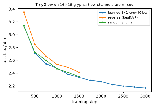
The learned 1×1 convolution and the random shuffle are neck and neck; both are clearly better than reverse at every checkpoint. The paper’s ordering is clearer. Our MLP couplings see the whole half-tensor and already mix a lot; with local CNN couplings the choice of mixing matters more.
Likelihood (code 05, part 1):
| model | bits/dim |
|---|---|
| uniform over 256 levels | 8.000 |
| independent pixels (a histogram per pixel) | 2.606 |
| TinyGlow, training images | 2.110 |
| TinyGlow, test images | 2.168 |
The flow saves 0.44 bits per pixel over per-pixel histograms, with no sign of memorization. Part of what remains is the dequantization bound itself: each 8-bit level becomes a 1/256-wide box with sharp edges, a tiny checkerboard, which §3 showed smooth flows fit imperfectly. (Flow++, Ho et al. 2019, replaced uniform noise by a learned “variational dequantization” for this reason.)
What does a likelihood measure? Per test image, bits/dim correlates +0.775 with the fraction of inked pixels:
| digit | 0 | 1 | 2 | 3 | 4 | 5 | 6 | 7 | 8 | 9 |
|---|---|---|---|---|---|---|---|---|---|---|
| bits/dim | 2.44 | 1.37 | 2.34 | 2.24 | 2.09 | 2.26 | 2.38 | 1.68 | 2.48 | 2.32 |
| inked fraction | 0.163 | 0.057 | 0.149 | 0.151 | 0.112 | 0.152 | 0.165 | 0.091 | 0.194 | 0.171 |
A likelihood counts how many bits it takes to describe an image, and here that is mostly “how much ink”. A “1” is twice as cheap as an “8”. High likelihood is not the same as typical. This is the root of a famous surprise: flows trained on CIFAR-10 assign higher likelihood to SVHN house numbers, which they never saw, because those images are simpler (Nalisnick et al. 2019).
Exploding inverses (code 05, part 2). We trained the same model for 1500 steps with three coupling scale functions:
| coupling scale | test bits/dim | round trip on test images | inf/NaN samples at T = 1 (of 2000) | at T = 0.8 |
|---|---|---|---|---|
| tanh-bounded log-scale, |log s| < 1.5 (ours) | 2.333 | — | 0 (main model) | 0 |
| sigmoid(raw + 2) (Glow’s code) | 2.441 | 4.9e−5 | 137 | 12 |
| additive, s = 1 (NICE) | 3.073 | 5.5e−6 | 0 | 0 |
- Glow’s sigmoid scale is a few hundredths of a bit worse, and its inverse explodes. Data → latent → data round trips are exact, yet 7% of samples overflow float32. The sigmoid lets a coupling contract a coordinate almost to zero for some inputs. That is harmless on training data. At a latent far from where the data map, the inverse divides by such a tiny scale, and a few such steps in a row overflow. Invertible on paper is not invertible in floating point (Behrmann et al. 2021 study these “exploding inverses”).
- Bounding the log-scale caps every inverse step at e^1.5. It removed the problem and was even a little better in likelihood.
- Additive coupling is stable but much worse: all per-pixel rescaling must come from ActNorm and the 1×1 convolutions, which act on whole channels.
4.6 Temperature, interpolation, manipulation
Temperature (code 05, part 3). 2000 samples per T, scored by Lecture 3’s Judge:
| T | recognizable | valid | class entropy (bits) | mini FID | nearest real | inked fraction |
|---|---|---|---|---|---|---|
| 1.0 | 0.726 | 0.630 | 3.15 | 248 | 0.088 | 0.100 |
| 0.8 | 0.701 | 0.663 | 3.04 | 449 | 0.082 | — |
| 0.7 | 0.686 | 0.667 | 2.93 | 565 | 0.080 | 0.082 |
| 0.6 | 0.671 | 0.654 | 2.82 | 682 | 0.078 | — |
| 0.5 | 0.653 | 0.642 | 2.67 | 790 | 0.077 | 0.077 |
(Real images: recognizable 1.000, valid 0.989, FID 1.1, nearest real 0.064, inked fraction 0.139.)
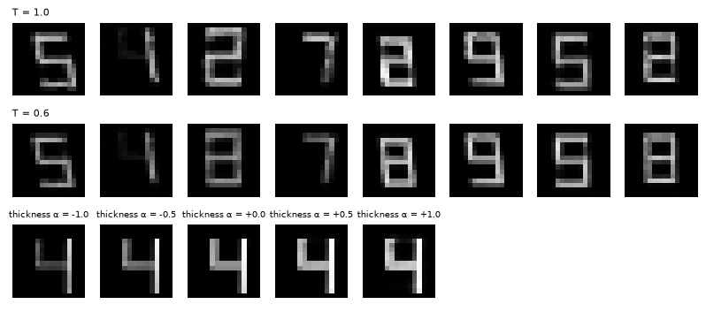
At T = 1 most samples are recognizable glyphs, but they are fainter than real ones, and the digit mix is off. Digits with many segments (0, 2, 6, 8) appear only 4–6% of the time instead of 10%. This is the likelihood–ink relation at work: ink is expensive, so a likelihood-trained flow spends little of it.
Lowering T does not help here, unlike on Glow’s faces:
- recognizability drops slowly and the valid rate barely moves;
- the class entropy and FID get worse, because the imbalance grows: at T = 0.5 the digits 0, 2, 6 and 8 almost vanish (≤ 1.4% each);
- low T moves samples toward the model’s high-density region, and for this model that region is “faint”.
Whether T < 1 improves samples depends on the data and on what you measure. The samples are as far from the training set as from unseen real images (0.088 vs 0.088): the flow is not copying.
For comparison with Lecture 3, the 8-D VAE reached FID 162 and valid 0.616 on the same Judge; the AE with a fitted Gaussian reached FID 53. The flow’s samples are better on validity but worse on FID: good likelihood does not guarantee good samples.
Interpolation (code 05, part 4). Midpoints between 300 pairs of test glyphs of the same digit:
| midpoint | recognizable | valid | same digit | nearest real | |z_mid| / |z_end| |
|---|---|---|---|---|---|
| pixel average | 0.950 | 0.553 | 0.997 | 0.103 | — |
| linear in z | 0.967 | 0.960 | 0.953 | 0.068 | 0.726 |
| spherical in z | 0.963 | 0.857 | 0.963 | 0.082 | 1.001 |
| (endpoints) | 1.000 | 0.980 | 1.000 | 0.064 | — |
- The pixel average keeps the digit but is a double image (Lecture 1 §4.3), valid only 55% of the time. Latent midpoints are single glyphs, at the price of changing the digit 4–5% of the time.
- The linear midpoint is a low-temperature point. Two random 256-D latents are nearly orthogonal, so their midpoint is about 1/√2 shorter (0.726): it lies inside the “soap bubble” where the Gaussian has almost no samples (P1 §2).
- Here that helps. Linear midpoints are the cleanest, almost as realistic as the real endpoints. The digit-imbalance problem of low T does not arise, because the two endpoints fix the digit.
A thickness direction (code 05, part 5). Following Glow’s recipe, we compute d = mean z(thickest quarter) − mean z(thinnest quarter) from 8000 training images, using the style factor “thick” that the flow never saw in training. Then we add α·d to the latents of 500 test images:
| α | −1.0 | −0.5 | 0 | +0.5 | +1.0 |
|---|---|---|---|---|---|
| inked fraction | 0.085 | 0.112 | 0.141 | 0.168 | 0.189 |
| same digit as before | 0.854 | 0.990 | 1.000 | 1.000 | 0.988 |
Real images: 0.109 for the thinnest quarter, 0.170 for the thickest.
α = ±0.5 lands on the real quartiles, and ±1 extrapolates beyond them. The digit survives moderate edits; thinning too far erases faint segments. The latent space was never trained to be disentangled, yet a difference of means finds a direction that is mostly “thickness” — the same recipe as smiling or blond hair on faces.
4.7 Limitations
- Sample quality. At equal compute, flow samples lag behind GANs (and later diffusion), and good bits/dim do not imply good samples (§4.5).
- Cost. The latent is as large as the image, and every layer must be invertible and keep its activations’ full dimension. Glow models are large and slow to train.
- Topology. A flow is still a deformed Gaussian. It cannot represent truly disconnected supports, or data on a lower-dimensional manifold, without extreme Jacobians (§3.3).
- Numerics. Invertibility in exact arithmetic can fail in floating point (§4.5).
5. Invertible residual networks (Behrmann et al. 2019)
5.1 Motivation: no special structure
Every flow so far designs its layers around the determinant: rank one, triangular, LU. Behrmann et al. ask a different question: can an ordinary ResNet block,
with g an arbitrary small network, be a flow? Its Jacobian I + J_g is a full D×D matrix, so the expressive power is not restricted by structure. If it works, the same architecture could serve both classification and density estimation. The paper presents i-ResNets as the first architecture to do well on both.
5.2 Invertibility from a Lipschitz constraint
Theorem. If g is a contraction, Lip(g) = c < 1, then F(x) = x + g(x) is invertible.
Proof sketch. For a given y, the preimages of y are the fixed points of T(x) = y − g(x). Since ‖T(a) − T(b)‖ = ‖g(a) − g(b)‖ ≤ c‖a − b‖, T is a contraction, so by Banach’s fixed-point theorem it has exactly one fixed point. Iterating x_{k+1} = y − g(x_k) converges to it, with error at most c^k times the initial error.
How to make Lip(g) < 1: if g = W_3 ∘ φ ∘ W_2 ∘ φ ∘ W_1 with 1-Lipschitz activations φ (ReLU, ELU), then Lip(g) ≤ Π‖W_i‖₂. Spectral normalization rescales each W_i so that its largest singular value is at most a chosen coefficient (the paper uses c = 0.9). The singular value is estimated by power iteration, one step per training iteration.
The same argument bounds both directions:
Each block can only stretch a little, so expressive i-ResNets need many blocks, and c close to 1 makes the inverse slow and numerically delicate.
Code 06, part 1.
- 1-D. With g(x) = c·sin x, fixed-point iteration solves f(x) = 2 to 1e−8 in 6, 15 and 19 iterations for c = 0.5, 0.9, 0.99. With c = 1.5, f is not monotone and the iteration never settles.
- 64-D random blocks reach float32 precision within 10 iterations for every c. The rate c^k is a worst case, and freshly initialized blocks stretch far less than their bound.
- Trained blocks use their budget (part 3): after 20 iterations their residual is 1e−2 to 2e−1 for c ≥ 0.9.
5.3 The log-determinant as a power series
For a matrix A with ‖A‖ < 1, log det(I + A) = tr log(I + A), and the matrix logarithm has the same series as log(1 + x):
Two approximations make this affordable:
- Truncate after n terms. The error is bounded by D·Σ_{k>n} c^k/k = −D·(log(1 − c) + Σ_{k≤n} c^k/k) (the paper’s bound; exercise 8). It decays like c^n: fast for c = 0.5, slowly for c near 1.
- Hutchinson’s estimator tr(A) = E_v[vᵀAv] for any random v with E[vvᵀ] = I. Then vᵀJ_g^k v needs only k vector–Jacobian products. No Jacobian matrix is ever formed, and the cost per sample is that of a few backward passes, for any D.
The resulting estimate is unbiased for the truncated series but biased overall. The gradient is obtained by backpropagating through the estimator.
Code 06, part 2. We use a linear residual branch g(x) = A·x whose 64 eigenvalues are spread evenly over [−c, c], so the exact log-det is Σ log(1 + λ_i).
| c | exact log|det| | truncation bias, 10 terms | 50 terms | std of one Hutchinson estimate |
|---|---|---|---|---|
| 0.5 | −2.995 | +0.0001 | +0.0000 | 3.2–3.8 |
| 0.9 | −13.11 | +0.40 | +0.0009 | 6.4–8.7 |
| 0.99 | −20.15 | +2.97 | +0.59 | 6.8–11.6 |
- Truncation bias is controlled by the eigenvalues near ±c. The log(1 + λ) for λ ≈ −0.99 is −4.6, and its series converges very slowly.
- The truncated series overestimates the log-det — here every missing term is negative — so a truncated estimator is biased toward higher likelihood.
- One Hutchinson vector is noisy, more so for larger c. That is acceptable for training (it averages over a minibatch), not for reporting a likelihood.
5.4 What the paper reports
- Density estimation. i-ResNets reach 1.06 bits/dim on MNIST and 3.45 on CIFAR-10. That is competitive with the flows of the time (RealNVP 3.49, Glow 3.35, FFJORD 3.40 on CIFAR-10) without any coupling or triangular structure.
- Classification. With the Lipschitz constraint, i-ResNets classify CIFAR-10 and ImageNet nearly as well as ordinary ResNets of the same depth: invertibility costs little discriminative accuracy.
- Generality. The same architecture can be trained as a hybrid model, one network that both classifies and estimates densities.
5.5 Our experiments
Code 06, part 3 trains i-ResNets on the same ring as §3, with the exact 2×2 log-det unless stated (1500 steps of 256 fresh points):
| model | parameters | KL | low-density | Lipschitz bound | inverse residual after 20 / 100 iterations |
|---|---|---|---|---|---|
| 8 blocks, c = 0.5 | 35,856 | 0.698 | 0.288 | 0.525 | 2.2e−6 / 2.2e−6 |
| 8 blocks, c = 0.9 | 35,856 | 0.184 | 0.071 | 0.910 | 1.5e−2 / 6.6e−6 |
| 8 blocks, c = 0.97 | 35,856 | 0.132 | 0.042 | 1.008 | 8.7e−2 / 2.0e−3 |
| 8 blocks, c = 0.9, series (5 terms + Hutchinson) | 35,856 | 0.363 | 0.128 | 0.922 | 2.2e−1 / 2.0e−5 |
| 16 blocks, c = 0.9 | 71,712 | 0.053 | 0.026 | 0.909 | 1.1e−2 / 6.7e−6 |
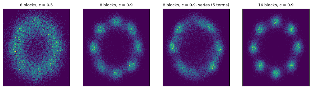
- c = 0.5 is too timid. Eight small moves cannot separate eight modes; the figure shows a blurry annulus.
- Larger c helps, and so does depth. 16 blocks with c = 0.9 reach a lower KL than the 12-coupling RealNVP of §3.2 (0.053 vs 0.095), with a third of the parameters and fewer steps, though with slightly more low-density samples (0.026 vs 0.019). A free-form Jacobian is expressive, if you can afford its determinant.
- The paper’s estimator is clearly worse at the same budget (KL 0.363 vs 0.184): noisier and biased gradients. In 2-D the exact determinant is cheap; the estimator exists for images, where J_g is thousands × thousands.
- The Lipschitz constraint is only approximate. One power iteration per step lags behind the moving weights; with c = 0.97 the measured bound reached 1.008, and invertibility is then no longer guaranteed. Larger c also makes the inverse slower.
5.6 Where this went
- Residual Flows (Chen et al. 2019) removed the truncation bias by drawing the number of terms at random (“Russian roulette” estimator) and introduced better Lipschitz activations.
- Continuous-time flows. A residual block x + g(x) is one Euler step of the ODE dx/dt = g(x). Neural ODEs and FFJORD (Chen et al. 2018; Grathwohl et al. 2019) take the limit: a flow defined by an ODE, whose log-det obeys d log p/dt = −tr(∂g/∂x), again estimated with Hutchinson’s trick. They removed the architectural constraints, but training required solving ODEs at every step.
- Flow matching (Lecture 16) keeps the ODE but trains the velocity field by simple regression, without simulating anything — the idea that finally made continuous flows practical at scale.
6. The big picture
6.1 Flows in the five-component framework
| Component | VI flows (Rezende & Mohamed) | Glow | i-ResNet |
|---|---|---|---|
| formulation | posterior = Gaussian pushed through K maps | data = invertible map of a Gaussian, multi-scale | data = invertible ResNet of a Gaussian |
| representation | planar / radial layers | ActNorm, LU 1×1 conv, affine coupling with CNNs | spectrally normalized residual blocks |
| objective | ELBO with exact log q | exact log-likelihood (dequantized), bits/dim | exact log-likelihood, estimated log-det |
| optimization | SGD + reparameterization + annealing | SGD; data-dependent init; zero-init couplings | SGD through a stochastic log-det |
| inference | samples and log q of q | sampling in one pass; exact encoding; temperature | density in one pass; sampling by fixed-point iteration |
6.2 Flows vs VAEs
| VAE (Lecture 3) | Flow | |
|---|---|---|
| likelihood | lower bound (ELBO) | exact |
| latent dimension | anything (usually ≪ D) | = D |
| encoder | approximate, learned separately | exact inverse of the generator |
| architecture | free | constrained (invertible, cheap log-det) |
| typical samples | blurry | sharp but speckled / off-balance (§4.6) |
The two ideas meet in the middle. A VAE can use a flow as its posterior (§2) or as its prior. A flow can use a VAE-like learned dequantization (Flow++).
6.3 Why this lecture matters later
- Lecture 5–6 (autoregressive models). An autoregressive model is a flow with a triangular Jacobian. MAF and IAF make that literal, and the MAF/IAF speed trade-off is §1.3’s table made sharp.
- Lecture 12 (diffusion). Every diffusion model has a probability-flow ODE: a continuous normalizing flow with the same marginals. That ODE gives exact likelihoods for diffusion models, through §5.6’s machinery.
- Lecture 16 (flow matching). It trains a continuous flow without ever computing a log-determinant.
- Tokenizers and latent spaces (Lectures 7–8). Glow’s lesson that “a learned latent space supports interpolation and attribute arithmetic” is now everyday practice, usually with VAE latents instead of flow latents.
7. Summary
- A flow is an invertible generator. With x = g(z) invertible, log p(x) = log p_Z(f(x)) + log|det ∂f/∂x| holds exactly. Compositions add their log-dets. Which direction must be cheap depends on the job: VI only needs latent → data, density estimation needs data → latent.
- Three costs. The determinant must be cheap by construction; invertibility must be guaranteed by parameterization; dimension and topology are preserved. A Gaussian on a smooth rubber sheet cannot be cut into islands, so flows leave bridges between modes — and our ring flow learned to put them where the base has little mass.
- Rezende & Mohamed: planar (rank-one) and radial flows with O(D) log-dets turn a Gaussian posterior into a flexible one.
- With annealing, 8 one-dimensional planar layers cut Lecture 3’s bimodal gap from 0.737 to about 0.001 nat in 2 of 3 runs.
- Without annealing, the reverse KL makes them lock onto one mode at a cost of about log 2. Richer families fix capacity, not optimization.
- Coupling layers (NICE / RealNVP) keep half the input and affinely transform the rest. The Jacobian is triangular, the inverse is free, and the inner network can be anything.
- Glow: ActNorm (data-dependent init), an invertible 1×1 convolution with an O(C) log-det via LU, and zero-initialized affine couplings, in a multi-scale architecture.
- In our glyph experiments the learned 1×1 conv tied with a shuffle and beat reverse.
- Glow’s sigmoid scale made 7% of samples explode in float32.
- Likelihood tracked ink, not typicality.
- Temperature did not help, but linear latent interpolation and a difference-of-means thickness direction worked.
- i-ResNets: y = x + g(x) is invertible when Lip(g) < 1 (Banach). The inverse comes from fixed-point iteration; the log-det from a truncated power series with Hutchinson traces.
- Larger c is more expressive but slower to invert and harder to estimate.
- The Lipschitz constraint is only approximately enforced.
- In 2-D, 16 blocks beat a RealNVP three times their size.
8. Common pitfalls
- “A flow can map a Gaussian onto any distribution.” Only onto distributions that are smooth deformations of a Gaussian. Disconnected supports and lower-dimensional manifolds are only approximable, with bridges and huge Jacobians (§3.3).
- “The log-likelihood of a flow is a bound, like the ELBO.” For continuous data it is exact. For discrete images it is a bound only because of dequantization (§4.3).
- “Invertible means I can always sample.” Invertible in exact arithmetic, yes. In float32, contracting layers can make the inverse explode (§4.5), and ill-conditioned 1×1 convolutions lose precision (§4.2).
- “Higher likelihood means more typical images.” Likelihood counts description length. Simple images (fewer lit pixels, SVHN vs CIFAR) get higher likelihood even when they are atypical or never seen (§4.5).
- “Lower temperature gives better samples.” It gives different samples: more typical, less diverse, sometimes unbalanced (§3.4, §4.6).
- “Planar flows can make any posterior.” In principle with many layers; in practice reverse KL and optimization decide (§2.4), and planar layers scale poorly to high dimensions.
- “Coupling layers are weak because each changes only half the input.” Alternation, mixing (1×1 convolutions) and arbitrary inner networks make stacks of couplings very expressive. They are the backbone of most practical flows.
- “Spectral normalization guarantees Lip(g) < 1.” Only if the power iteration has converged; with one step per update the bound can be exceeded (§5.5).
- “The power-series log-det is unbiased.” Hutchinson makes each trace unbiased, but truncation biases the sum, toward higher likelihood in our test (§5.3).
9. Exercises
Exercise 1 (planar flows). (a) Prove the matrix determinant lemma det(I + uvᵀ) = 1 + vᵀu. (b) For f(z) = z + u tanh(wᵀz + b), show that f is invertible iff wᵀu ≥ −1. (Hint: decompose z into the component along w and the rest; f only changes the scalar wᵀz monotonically iff …) (c) Show that wᵀû = m(wᵀu) > −1 for the paper’s û.
Answer
(a) I + uvᵀ has eigenvalue 1 on the (D−1)-dimensional subspace orthogonal to v (for such x, (I + uvᵀ)x = x). Restricted to the remaining direction, the eigenvalue is 1 + vᵀu: (I + uvᵀ)u = (1 + vᵀu)u. The determinant is the product of eigenvalues. (For the degenerate case u ⊥ v, all eigenvalues are 1 and the formula still holds.)
(b) Write a = wᵀz. Then wᵀf(z) = a + (wᵀu) tanh(a + b) =: φ(a), and f(z) = z + u tanh(a + b) depends on z only through z itself and a.
- If φ is strictly increasing, then given y = f(z) we can recover a from wᵀy = φ(a), then z = y − u tanh(a + b). So f is invertible.
- φ′(a) = 1 + (wᵀu)(1 − tanh²(a + b)) ranges over (1, 1 + wᵀu] or [1 + wᵀu, 1) as tanh² ranges over [0, 1). It is positive everywhere iff 1 + wᵀu ≥ 0. At wᵀu = −1 it is zero only at a single point, which still leaves φ strictly increasing.
- If wᵀu < −1, φ decreases near a = −b, so two values of a give the same wᵀy, and f is not injective.
(c) wᵀû = wᵀu + (m(wᵀu) − wᵀu)·wᵀw/‖w‖² = m(wᵀu) = −1 + log(1 + e^{wᵀu}) > −1, since log(1 + e^x) > 0.
Exercise 2 (radial flows). For f(z) = z + βh(r)(z − z₀) with h = 1/(α + r), derive det ∂f/∂z = (1 + βh)^{D−1}(1 + βh + βh′r).
Answer
Let e = (z − z₀)/r. Then ∂f/∂z = (1 + βh)I + βh′(r)·(z − z₀)eᵀ = (1 + βh)I + βh′ r · eeᵀ.
- Directions orthogonal to e have eigenvalue 1 + βh (D − 1 of them).
- e itself has eigenvalue 1 + βh + βh′r.
The product of eigenvalues gives the formula.
Exercise 3 (coupling layers). For y_a = x_a, y_b = x_b ⊙ exp(s(x_a)) + t(x_a): (a) write the Jacobian in block form and its log-determinant; (b) write the inverse; (c) explain why s and t can be non-invertible networks; (d) why must consecutive layers change which part is kept?
Answer
(a) The Jacobian is
which is block lower-triangular. So log|det| = Σ_j s_j(x_a).
(b) x_a = y_a and x_b = (y_b − t(y_a)) ⊙ exp(−s(y_a)).
(c) They are only ever evaluated at x_a (= y_a), never inverted. Their own Jacobians appear only in the off-diagonal block, which does not affect the determinant.
(d) Otherwise x_a would never change, and the composition would leave half the input untouched.
Exercise 4 (Glow’s layers). (a) Show that ActNorm on an H×W×C tensor has log|det| = H·W·Σ_c log|s_c|. (b) Show that a 1×1 convolution with matrix W has log|det| = H·W·log|det W|. (c) With W = PL(U + diag(s)), show that log|det W| = Σ log|s_c|.
Answer
(a) The Jacobian is diagonal, with s_c repeated H·W times for each channel.
(b) Reorder the coordinates pixel by pixel. The Jacobian is block-diagonal with H·W copies of W, so its determinant is (det W)^{HW}.
(c) det P = ±1 and det L = 1 (unit diagonal). U + diag(s) is upper-triangular with diagonal s, so its determinant is Π s_c.
Exercise 5 (directions). A flow is written in the generative direction, x = g(z) = g_K ∘ … ∘ g_1(z). Write log p_X(x) using only the forward Jacobians of the g_k evaluated at the intermediate points. Which intermediate points do you need, and how would you get them for a given data point x?
Answer
with z_K = x and z_{k−1} = g_k⁻¹(z_k). For a given x you must run the inverses backwards to get z_{K−1}, …, z_0. That is cheap for coupling layers, iterative for i-ResNets, and impossible in closed form for planar flows — which is why planar flows are used for VI, where the z_k come for free from the forward pass.
Exercise 6 (dequantization). Let k ∈ {0, …, 255}^D and y = (k + u)/256 with u ~ U(0,1)^D. For any continuous density p on [0, 1]^D, define P(k) = ∫ over the cube of k of p(y) dy. Show that log P(k) ≥ E_u[log p((k+u)/256)] − D log 256, and that Σ_k P(k) = 1.
Answer
P(k) = 256^{−D} · E_u[p((k+u)/256)], since the cube has volume 256^{−D} and u is uniform on it. By Jensen’s inequality (log is concave), log P(k) = log E_u[p] − D log 256 ≥ E_u[log p] − D log 256. The cubes tile [0, 1]^D, so the P(k) sum to ∫p = 1. Equality holds iff p is constant on each cube — which is why sharp cube edges matter (§4.5).
Exercise 7 (topology). (a) In 1-D, show that a continuous bijection g: ℝ → ℝ maps the interval [−1, 1] onto an interval. (b) Conclude that if p_Z is positive on ℝ, a continuous invertible g cannot produce a density that is zero on (−0.1, 0.1) and positive on both sides. (c) What can it do, and what does that cost in log|g′|?
Answer
(a) A continuous injective function on an interval is strictly monotone, and by the intermediate value theorem it attains every value between g(−1) and g(1).
(b) The image of ℝ is an interval containing points on both sides of (−0.1, 0.1), hence containing (−0.1, 0.1). Every point there is g(z) for some z where p_Z(z) > 0. The density there is p_Z(z)/|g′(z)| > 0.
(c) It can make |g′| enormous on the preimage of (−0.1, 0.1), so that the density there is tiny. If the preimage interval has length ℓ and must cover 0.2 units of x, then the average g′ there is 0.2/ℓ. A small mass needs a small ℓ, hence large log-derivatives. These are the steep Jacobians at the bridges of §3.3.
Exercise 8 (i-ResNet). (a) Prove that F(x) = x + g(x) with Lip(g) = c < 1 is injective and that Lip(F⁻¹) ≤ 1/(1 − c). (b) Show E[vᵀAv] = tr(A) when E[vvᵀ] = I. (c) Show that truncating the series after n terms makes an error of at most D·Σ_{k>n} c^k/k = −D(log(1 − c) + Σ_{k≤n} c^k/k).
Answer
(a) ‖F(a) − F(b)‖ ≥ ‖a − b‖ − ‖g(a) − g(b)‖ ≥ (1 − c)‖a − b‖. So F(a) = F(b) forces a = b, and for y = F(a), y′ = F(b) we get ‖F⁻¹(y) − F⁻¹(y′)‖ ≤ ‖y − y′‖/(1 − c).
(b) E[vᵀAv] = E[tr(Avvᵀ)] = tr(A E[vvᵀ]) = tr(A).
(c) |tr(J^k)| ≤ D‖J‖^k ≤ D c^k, because each of the D eigenvalues of J^k has modulus at most ‖J‖^k. Summing the tail gives D Σ_{k>n} c^k/k, and Σ_{k≥1} c^k/k = −log(1 − c).
Exercise 9 (hands-on).
(a) In 01_planar_radial_vi.py, turn the annealing off (β = 1 throughout). Which targets suffer most?
(b) In 03_coupling_flows.py, train the 12-coupling ring model with s_max = 1 instead of 3 (set layer.s_max after construction). How do the KL and the low-density share change? Why?
(c) In 05_glow_glyphs.py, compute the thickness direction from the first 1000 training images only. Does it still work?
(d) In 06_iresnet.py, train 16 blocks with c = 0.97. Is the extra expressiveness worth the slower inverse?
Answer (sketch)
(a) Expect the multi-part targets (U1’s two lobes, U3’s split bands) to suffer most: without annealing q locks onto whichever part it reaches first (compare §2.4).
(b) A tighter scale bound limits how strongly each coupling can stretch. The bridges need large stretches, so expect more low-density mass, although each layer becomes more stable. Your run decides how much.
(c) Usually yes. A difference of two means of 250 latents each is still a decent estimate of the direction, just noisier; the digit agreement at α = ±1 may drop.
(d) Compare the KL against the inverse residual. In our 8-block runs, c = 0.97 lowered KL from 0.184 to 0.132 but left a residual of 2e−3 after 100 iterations, and its measured Lipschitz bound exceeded 1.
10. Further reading
The required and optional papers
- D. Rezende & S. Mohamed, Variational Inference with Normalizing Flows, ICML 2015.
- D. P. Kingma & P. Dhariwal, Glow: Generative Flow with Invertible 1×1 Convolutions, NeurIPS 2018.
- J. Behrmann, W. Grathwohl, R. T. Q. Chen, D. Duvenaud, J.-H. Jacobsen, Invertible Residual Networks, ICML 2019.
- L. Weng, Flow-based Deep Generative Models (blog, 2018).
Background and follow-ups
- L. Dinh, D. Krueger, Y. Bengio, NICE: Non-linear Independent Components Estimation, 2014; L. Dinh, J. Sohl-Dickstein, S. Bengio, Density Estimation using Real NVP, ICLR 2017: coupling layers.
- D. P. Kingma et al., Improved Variational Inference with Inverse Autoregressive Flow, NIPS 2016; G. Papamakarios et al., Masked Autoregressive Flow for Density Estimation, NIPS 2017: autoregressive flows (Lecture 6).
- C. Durkan et al., Neural Spline Flows, NeurIPS 2019: much more expressive coupling functions.
- J. Ho et al., Flow++, ICML 2019: variational dequantization.
- R. T. Q. Chen et al., Neural Ordinary Differential Equations, NeurIPS 2018; W. Grathwohl et al., FFJORD, ICLR 2019: continuous-time flows.
- R. T. Q. Chen et al., Residual Flows for Invertible Generative Modeling, NeurIPS 2019: unbiased log-det estimation.
- E. Nalisnick et al., Do Deep Generative Models Know What They Don’t Know?, ICLR 2019: likelihood vs typicality.
- J. Behrmann et al., Understanding and Mitigating Exploding Inverses in Invertible Neural Networks, AISTATS 2021.
- G. Papamakarios et al., Normalizing Flows for Probabilistic Modeling and Inference, JMLR 2021; I. Kobyzev, S. Prince, M. Brubaker, Normalizing Flows: An Introduction and Review of Current Methods, TPAMI 2021: surveys.
Related notes in this course
- Prerequisite P1 §2 (the soap bubble), §6 (change of variables), §7 (bits/dim and dequantization).
- Lecture 1 §5.3 (forward vs reverse KL); Lecture 3 §2–§3 (the ELBO gap that §2 closes).
11. Next lecture
Lecture 5: Autoregressive models (original lecture · 09/19).
Flows made the density exact by making the generator invertible. Autoregressive models make it exact by the chain rule of probability:
Every factor is a small, normalized conditional distribution, so there is no determinant at all — and no constraint on the architecture beyond “do not look ahead”. The price moves to sampling, which must go one element at a time. We will see:
- that the chain rule holds in any order, and why some orders are easier to learn;
- why training (teacher forcing) and sampling differ;
- how causal convolutions and causal attention compute all conditionals in one pass.
Lecture 6 then shows that an autoregressive model with Gaussian conditionals is a flow with a triangular Jacobian (MAF / IAF), closing the loop with this lecture.