Maps to: MIT 6.S978 Deep Generative Models (Fall 2024), Reading · Tue 10/22/2024 · Diffusion Models (student paper session). Required papers:
- J. Ho, T. Salimans, Classifier-Free Diffusion Guidance, NeurIPS 2021 Workshop on Deep Generative Models (arXiv 2207.12598);
- T. Salimans, J. Ho, Progressive Distillation for Fast Sampling of Diffusion Models, ICLR 2022;
- E. Hoogeboom, J. Heek, T. Salimans, simple diffusion: End-to-end diffusion for high resolution images, ICML 2023.
Optional: R. Rombach et al., High-Resolution Image Synthesis with Latent Diffusion Models (CVPR 2022); T. Karras et al., Elucidating the Design Space of Diffusion-Based Generative Models (EDM, NeurIPS 2022); A. Ramesh et al., Hierarchical Text-Conditional Image Generation with CLIP Latents (unCLIP, 2022); T. Chen, On the Importance of Noise Scheduling for Diffusion Models (2023); S. Dieleman, Diffusion is spectral autoregression (blog, 2024).
Basis: This session consisted of student presentations, with no published slides. The notes are organized around three practical problems of the DDPM built in Lecture 12 — it cannot be steered strongly toward a condition, it needs hundreds of steps, and it does not scale to high-resolution pixels — and the paper that answers each. Background the papers rely on is explained first: continuous-time notation, the ε / x / v parameterizations, DDIM, classifier guidance. Paper claims are labelled “the paper reports / argues”. All experiments were designed for these notes and run on a CPU, with 2-D mixtures (where every score is exact) and the glyph latents of Lecture 12. Several outcomes differed from what I expected and are reported as they came out:
- with clean labels, guidance only made the glyph model worse; it helped once labels were noisy or the model weak;
- guided DDIM overshoots beyond the class rather than sampling the “tilted” distribution;
- x-prediction failed in our MLP for lack of a skip connection;
- one-shot distillation slightly beat progressive distillation on our small problem;
- the second-order Heun sampler lost to Euler below ~17 steps.
Code:
code/lecture13/— 6 scripts + the shared modulepractical_diffusion.py. They run in 3–110 s. Reading time: 4–5 hours including running the code.
0. How to read this lecture
0.1 Where we are
Lecture 12 built a DDPM from first principles: a forward process that adds Gaussian noise, a network that predicts the noise, and an ancestral sampler that takes T = 1000 small steps back. On glyph latents it worked (valid 0.90). But three things stand between that model and a system like Stable Diffusion:
| problem | symptom in Lecture 12 | paper of this session | idea |
|---|---|---|---|
| control | the model is unconditional; a conditional one follows p(x | c) exactly, ambiguities included | Ho & Salimans: classifier-free guidance | extrapolate from the unconditional prediction toward the conditional one |
| speed | 100–1000 network evaluations per sample | Salimans & Ho: progressive distillation | teach a student to do two sampler steps in one, and repeat |
| resolution | the pixel-space MLP failed already at 16 × 16 | Hoogeboom et al.: simple diffusion | shift the noise schedule toward noisier levels, and spend capacity at low resolution |
The optional papers fill in the rest of the modern recipe: latent diffusion (generate in an autoencoder’s latent space), EDM (treat sampling as solving an ODE well, and precondition the network), unCLIP (generate in a CLIP embedding space first), and two views of the noise schedule (Chen; Dieleman).
0.2 Learning goals
- Use the continuous-time notation , log-SNR , and convert between ε-, x- and v-prediction; know which loss weighting each implies (§1).
- Derive classifier guidance and classifier-free guidance from Bayes’ rule; explain label dropout; explain why guided sampling is not sampling (§2).
- Derive progressive distillation’s target from DDIM; explain why ε-prediction breaks it and v-prediction does not (§3).
- Derive simple diffusion’s schedule shift from average pooling, and list its other ingredients (§4).
- Explain EDM’s view of samplers as ODE solvers, its preconditioning, and why v-prediction is a special case (§5).
- Connect the noise schedule to image spectra: why diffusion generates coarse structure first (§4.5).
0.3 Map
| Section | Content | Code |
|---|---|---|
| §1 | Continuous-time notation, parameterizations, DDIM | — |
| §2 | Classifier-free guidance | 01_cfg_2d.py, 02_cfg_glyphs.py |
| §3 | Progressive distillation | 03_distill_2d.py, 04_distill_glyphs.py |
| §4 | simple diffusion: noise schedules and resolution | 06_resolution_spectra.py |
| §5 | Optional readings: latent diffusion, EDM, Chen, unCLIP, spectral autoregression | 05_samplers.py, 06_resolution_spectra.py |
| §6 | The big picture | — |
1. Background: the language of the three papers
All three papers (and EDM, Chen, simple diffusion’s successors) write diffusion in continuous time with signal and noise scales. This section translates Lecture 12 into that language.
1.1 Continuous time and log-SNR
Time runs from data () to noise ():
Lecture 12’s discrete is here. The one number that describes a noise level is the log signal-to-noise ratio
Two schedules with the same λ at some t corrupt the data identically there; a schedule is just a map , and what matters is how much training and sampling time it spends at each λ (Lecture 12 §5.4 already found that the range of λ mattered more than the number of steps).
The papers of this session use the cosine schedule (Nichol & Dhariwal 2021): , , so . It runs from to ; implementations clip it. practical_diffusion.logsnr clips to , so at , — pure noise to four digits.
1.2 Three things the network can predict
Given , any one of three quantities determines the other two:
| the network outputs | its plain MSE equals | ||
|---|---|---|---|
| ε (DDPM, Lecture 12) | |||
| x | |||
| v (Salimans & Ho) |
(SNR .) The v identities: , and similarly for ε. The last column is Exercise 3.
Two consequences run through this lecture:
- Each parameterization is also a loss weighting. “Predict ε with a plain MSE” (Lecture 12’s ) is “predict x with weight SNR”, which ignores the noisiest levels. Choosing what to predict changes which noise levels the training cares about.
- Each divides by something. ε-prediction divides by α — harmless with many small steps, fatal for a model that must jump from pure noise in one step (§3). x-prediction divides by σ (only to get ) and, more importantly, must output the clean image itself even when the input is already almost clean. v-prediction divides by nothing.
1.3 DDIM: a deterministic sampler
Lecture 12’s ancestral sampler draws from the Gaussian posterior . Song, Meng & Ermon’s DDIM (2021) instead re-uses the predicted noise:
“Keep the same noise, change its amount.” No fresh randomness enters, so the whole sampler is a deterministic map from the starting noise to a sample. It is a discretization of the probability-flow ODE of Lecture 12 §8 — exactly Euler’s method in suitable variables (§5.2, checked in code 05 to 1e-11). A parameter η interpolates between DDIM (η = 0) and the ancestral sampler (η = 1); practical_diffusion.sample implements both.
That determinism is what progressive distillation needs: a deterministic map can be learned by regression.
2. Classifier-free guidance (Ho & Salimans)
2.1 Why a conditional model is not enough
A class-conditional diffusion model trained to maximize likelihood learns — all of it. If some training images labelled “dog” are blurry, ambiguous or barely contain a dog, the model reproduces that. For images, people prefer samples that are more typical of the condition than the data is: sharper, more obviously a dog. GANs had truncation for this (Lecture 10): sample the latent from a narrower distribution and trade diversity for fidelity. Diffusion models have no single latent to truncate. Two ideas filled the gap.
2.2 Classifier guidance (Dhariwal & Nichol 2021)
Train, next to the diffusion model, a classifier on noisy images at every noise level. Bayes’ rule on the noisy marginal gives
So adding the classifier’s gradient to an unconditional score gives a conditional score. Classifier guidance scales it: sample with the score (in ε-terms, , using from Lecture 12 §7.2). With w > 0 the samples are pushed toward images the classifier is sure about. Dhariwal & Nichol report that this let diffusion models beat BigGAN’s FID on ImageNet — the paper’s title, “Diffusion Models Beat GANs” — with the same fidelity/diversity dial as truncation.
The drawbacks Ho & Salimans list:
- a second network, trained on noisy inputs, so off-the-shelf classifiers cannot be used;
- the classifier’s input gradient is exactly what an adversarial attack follows, so better Inception scores might partly come from fooling classifier-like metrics rather than from better images.
2.3 The implicit classifier
Bayes’ rule again, solved for the classifier:
The noisy classifier’s gradient is the difference between the conditional and unconditional noise predictions. A conditional and an unconditional diffusion model together are a classifier — the implicit classifier. Substituting it into classifier guidance:
is the plain conditional model; the unconditional one; extrapolates away from the unconditional prediction. (Many implementations write , the “guidance scale”; Stable Diffusion’s default is here.)
Training: label dropout. Both predictions come from one network. During training, replace the label by a special null token ∅ with probability (0.1–0.2), so the same network learns and . Sampling costs two forward passes per step (batched together in practical_diffusion.predict).
Any parameterization. Because , and are affine in each other with the same (§1.2), guiding any one of them with the same gives the same sampler (Exercise 2).
Code 01, Part 1 checks the Bayes identity with exact scores of a Gaussian mixture (three overlapping 2-D classes): by finite differences equals to within at every noise level. Classifier guidance and CFG are the same vector field; CFG simply gets the classifier for free.
2.4 What guided sampling actually produces
A tempting reading: at the guided score is , so guidance samples the class distribution tilted toward confidently classified points. That would be true if the tilt were applied to the clean distribution and then noised. It is not. Guidance tilts every noisy marginal: . Raising densities to powers does not commute with adding noise, so this family is not the noising of any one distribution, and following it is not sampling the tilted target.
Code 01, Part 2 measures the difference with exact scores (class 0, 200 steps). Each cell reads tilted target / guided DDIM / guided ancestral:
| w | mean p(c | x) | spread (class: 0.500) | outside the class’s 99% disc |
|---|---|---|---|
| 0 | 0.936 / 0.937 / 0.939 | 0.500 / 0.500 / 0.493 | 0.010 / 0.011 / 0.008 |
| 1 | 0.968 / 0.999 / 0.991 | 0.471 / 0.390 / 0.442 | 0.006 / 0.009 / 0.008 |
| 4 | 0.985 / 1.000 / 0.998 | 0.451 / 0.326 / 0.433 | 0.006 / 0.081 / 0.015 |
| 8 | 0.990 / 1.000 / 0.999 | 0.440 / 0.303 / 0.432 | 0.006 / 0.566 / 0.022 |
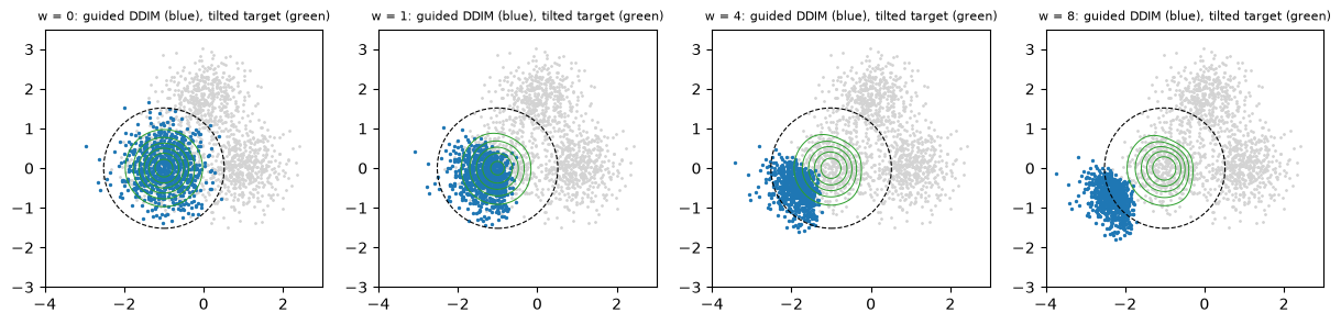
- Guidance does its job: samples become more class-like and less diverse as w grows — the fidelity/diversity trade-off.
- But it overshoots. The tilted target stays inside the class and narrows only a little. Guided DDIM narrows much more and, at w ≥ 4, pushes samples beyond the class, away from the other two. The guidance term is largest at high noise, where the classes still overlap, and a deterministic sampler never undoes an early push.
- The ancestral sampler overshoots far less: its fresh noise and the score’s pull toward the data act as a corrector at every step. Recent analyses make “CFG is not the tilted distribution” precise (Chidambaram et al. 2024; Bradley & Nakkiran 2024, who describe CFG as a kind of predictor–corrector).
In images, this overshoot is the familiar look of over-guided samples: over-saturated colours, exaggerated features. We will see thicker strokes on glyphs.
Part 3 trains one network with label dropout (0.1) instead of using exact scores. Its guided samples follow the exact ones in confidence and spread (at w = 1: p(c | x) 0.999 vs 0.999, spread 0.373 vs 0.390). The overshoot at w = 4 is smaller (1.6% outside vs 8.1%), because it happens far from the data, where the network is least accurate. The null label alone generates the three classes in proportions 0.326 / 0.334 / 0.340.
2.5 Experiment: guidance on glyphs
Code 02 trains a class-conditional latent diffusion model (v-prediction, cosine schedule, the 64 glyph latents of Lecture 12) with and samples 200 glyphs per digit with DDIM (64 steps). Besides the Judge’s columns, on-class is the fraction confidently read as the requested digit, and style spread the standard deviation of the ink amount within a digit (real glyphs: 0.0261) — a proxy for the variety of stroke widths and sizes.
Clean labels. I expected the textbook curve — FID first improves with w, then degrades. It did not:
| w | valid | FID | on-class | style spread | ink (real 0.136) |
|---|---|---|---|---|---|
| unconditional (∅) | 0.741 | 32.66 | 0.079 | 0.0444 | 0.134 |
| 0 | 0.993 | 3.68 | 0.998 | 0.0232 | 0.136 |
| 0.5 | 0.994 | 6.61 | 1.000 | 0.0217 | 0.141 |
| 1 | 0.989 | 15.92 | 1.000 | 0.0212 | 0.145 |
| 2 | 0.972 | 43.12 | 1.000 | 0.0212 | 0.152 |
| 4 | 0.915 | 116.66 | 1.000 | 0.0228 | 0.162 |
The plain conditional model is already excellent: valid as high as real glyphs, FID 3.7, the requested digit 99.8% of the time. Seven-segment classes never overlap: every real glyph is unambiguously one digit, so on the data and the tilted distribution equals . Guidance has nothing to correct, and only its side effect remains: pushing away from the other digits at high noise thickens the strokes (ink 0.136 → 0.162) and steadily worsens FID. The unconditional branch, trained on 10% of the examples, is much worse than the conditional one.
Noisy labels. Real data are not like that: captions and labels describe images only partly. To mimic this, 30% of the training labels are replaced by random digits (27% end up wrong). Now :
| w | valid | FID | on-class | style spread |
|---|---|---|---|---|
| 0 | 0.927 | 8.24 | 0.677 | 0.0346 |
| 0.5 | 0.972 | 2.87 | 0.894 | 0.0282 |
| 1 | 0.982 | 4.96 | 0.968 | 0.0243 |
| 2 | 0.982 | 22.19 | 0.997 | 0.0219 |
| 4 | 0.953 | 78.12 | 1.000 | 0.0215 |
At w = 0 a third of the samples are not the requested digit. Guidance re-weights by the implicit classifier , and the wrong digits disappear: on-class reaches 0.997 by w = 2. FID is U-shaped with its best value at w = 0.5, while the style spread falls steadily. This is the trade-off of the CFG paper.
A weak model. An under-fit model (width 128, 1500 steps) shows the same pattern for a different reason: guidance compensates for the model’s own blurriness. With , FID goes 30.8 → 13.5 → 21.9 → 63.3 for w = 0 / 0.5 / 1 / 2, and on-class 0.871 → 0.963 → 0.986 → 0.996. Changing the dropout rate:
| p_uncond | valid at w = 0 / 0.5 / 1 / 2 | FID at w = 0 / 0.5 / 1 / 2 |
|---|---|---|
| 0.1 | 0.750 / 0.855 / 0.882 / 0.845 | 30.8 / 13.5 / 21.9 / 63.3 |
| 0.2 | 0.703 / 0.801 / 0.813 / 0.773 | 33.2 / 16.7 / 24.1 / 61.6 |
| 0.5 | 0.568 / 0.680 / 0.708 / 0.665 | 45.3 / 23.4 / 24.8 / 53.0 |
0.1 and 0.2 behave alike; 0.5 starves the conditional model (lower validity and on-class at every w).
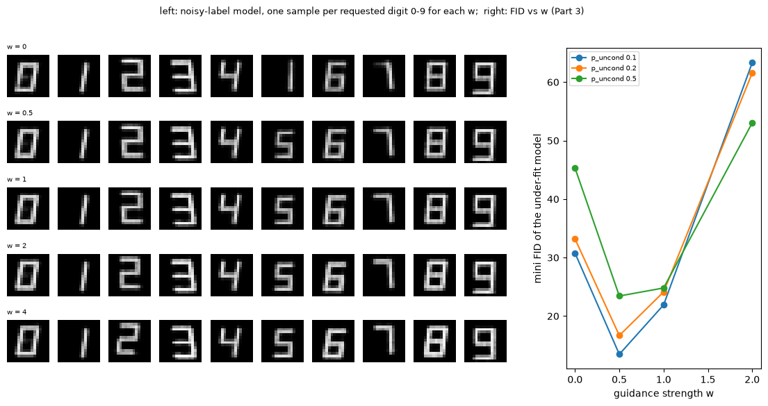
The lesson. Guidance is a correction for the gap between what the model learned and what we want: noisy conditioning data, or a model too weak to represent sharply. Large text-to-image models live in exactly that regime (web captions are noisy, prompts are open-ended), which is why they use large guidance scales. When there is no gap, guidance has only its cost.
2.6 What the paper reports
Ho & Salimans train class-conditional models on ImageNet 64×64 and 128×128 and sweep w and . They report:
- Inception Score rises steadily with w, while FID is best at a small guidance strength (around w = 0.1–0.3) and worsens beyond — the same U-shape as our noisy-label model;
- works better than 0.5 — only a small share of the model’s capacity is needed for the unconditional task;
- samples become visibly less diverse and more saturated at large w.
Their conclusion is that a pure generative model, with no classifier anywhere, can produce the quality/diversity trade-off that classifier guidance produced. They also note a limitation: two forward passes per step slow sampling down. Guided distillation (Meng et al. 2023) later folds the guided teacher into a single student.
2.7 Guidance in practice
CFG became the default way to condition diffusion models on text (GLIDE, Imagen, Stable Diffusion, DALL·E 2’s decoder, video models). Common practice adds a few variations:
- negative prompts: replace ∅ by an unwanted condition, so guidance pushes away from it;
- guidance intervals: apply guidance only at intermediate noise levels, because §2.4’s overshoot comes mainly from the noisiest levels;
- rescaling: renormalize the guided prediction to limit saturation.
All are heuristics around the same formula.
3. Progressive distillation (Salimans & Ho)
3.1 The cost problem, and why DDIM helps
Lecture 12’s DDPM needed ~100 steps for good samples (FID 36.7 at 100, 72.7 at 20 on glyphs). Each step is a full network evaluation, so a diffusion model is ~100× more expensive to sample than a GAN of the same size. Better ODE solvers (§5.2) help down to a few tens of steps. Below that, every solver fails for a structural reason: one deterministic step from pure noise can only land on , the mean of the data. The sampler is not wrong; the network is answering a different question (the conditional mean) from the one we need (a map from noise to one particular sample).
DDIM’s determinism suggests the fix. With N steps, DDIM is a fixed function . If is a good sampler, train a new network whose -step DDIM reproduces . That changes what the network predicts at each step: no longer the conditional mean, but whatever makes the coarse step land where two fine steps would.
3.2 The algorithm
The student starts as a copy of the teacher (sampled with steps). For a training example:
- draw , a student time (), and noise it: ;
- run two teacher DDIM steps, , reaching ;
- find the for which one DDIM step from lands exactly on :
- take a gradient step on .
When the student has converged, it becomes the teacher, is halved, and the process repeats: 1024 → 512 → … → 4 → 2 → 1. (Edge case: when the teacher’s second step already returns its , so is that; the formula with , agrees.) practical_diffusion.distill_round implements one round.
Why rounds instead of one jump? Each round is a small change to a network that already works. The student starts from the teacher’s weights, and its target differs from what it already does by the error of one halving. The paper argues that this keeps each round cheap, and reports that the whole procedure costs no more than training the original model.
3.3 The parameterization: why ε breaks and v works
At the end of distillation the student’s single step starts from — essentially pure noise, — and must output a good . With ε-prediction, : an error δ in becomes an error δ/α in . With our schedule that is a factor 1/α₁ = 1808. As SNR → 0, ε-prediction stops carrying information about x at all: predicting the noise from (almost) pure noise is trivial, and x is the tiny remainder.
The paper considers three alternatives, all well behaved at SNR = 0:
- predict x directly;
- predict x and ε with two output channels, and mix them by the SNR;
- predict v , which equals at and at , and from which divides by nothing.
They pair these with a loss weighting expressed in x-space: “truncated SNR”, , or “SNR + 1”, which is exactly v-prediction’s plain MSE (§1.2). The paper reports that these choices train the original (undistilled) model about as well as ε-prediction, and that only they survive distillation. v-prediction has since become standard (Imagen Video, Stable Diffusion 2’s 768-px model, and others).
3.4 Experiment: distillation in 2-D
Code 03 trains teachers on Lecture 9’s ring of 8 Gaussians (std 0.05, radius 2) with each parameterization. It then distills 128 → 64 → … → 1 step, 500 updates per round. “Quality” is the fraction of samples within 3 std of a mode. Each cell reads DDIM with the teacher / the distilled student:
| steps | v-prediction | x-prediction (truncated SNR) | ε-prediction |
|---|---|---|---|
| 128 (teacher) | 0.929 | 0.280 | 0.964 |
| 16 | 0.915 / 0.925 | 0.231 / 0.255 | 0.286 / 0.864 |
| 8 | 0.826 / 0.918 | 0.209 / 0.251 | 0.090 / 0.298 |
| 4 | 0.541 / 0.890 | 0.125 / 0.250 | 0.015 / 0.011 |
| 2 | 0.007 / 0.851 | 0.023 / 0.231 | 0.001 / 0.004 |
| 1 | 0.000 / 0.814 | 0.000 / 0.210 | 0.000 / 0.002 |
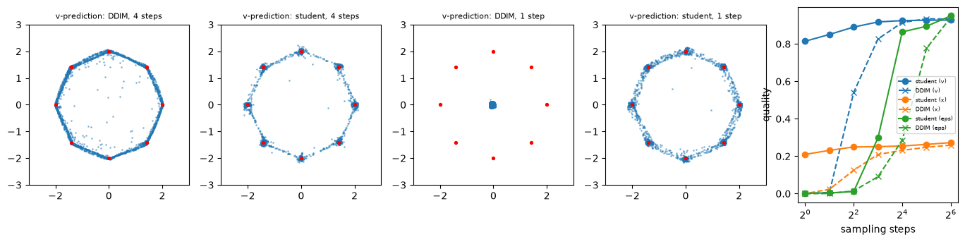
- DDIM collapses below ~8 steps. At 4 steps its samples fall on the straight lines between modes (the figure’s octagon); at 1 step all of them land at the centre of the ring, .
- The v-student works at every step count. Even with 1 step it covers all 8 modes with quality 0.81, and its samples stay within 0.09 of the 128-step teacher’s from the same noise. Total distillation cost: 7 × 500 = 3500 updates, less than the teacher’s own 4000.
- ε breaks, as the paper argues, in two places. The ε teacher’s own DDIM drifts already at 64 steps: its samples land 0.87 away from its 128-step ones, and quality collapses below 32 steps — the first step multiplies the ε error by 1808. Distillation rescues it down to 16 steps (0.864) and fails from 8 steps on.
- x failed for a reason I had not planned. Its teacher was already poor (quality 0.28), with plain MSE and with the paper’s truncated-SNR weighting alike. An x-predicting network must output the clean point even when its input is already almost clean. Near t = 0 it must reproduce its own input to within the modes’ width (0.05), and an MLP without a skip connection does not. v-prediction has that skip built in: as . This is the idea EDM formalizes as preconditioning (§5.2). The paper’s U-Nets, whose skip connections make the identity map easy, distill fine with x.
3.5 Experiment: distilling the glyph generator
Code 04 distills script 02’s clean-label glyph model (64 DDIM steps, FID 3.52 from this set of noises) in six rounds of 1000 updates:
| steps | 32 | 16 | 8 | 4 | 2 | 1 |
|---|---|---|---|---|---|---|
| DDIM, FID | 3.95 | 5.15 | 8.38 | 19.5 | 47.0 | 226 |
| DDIM, style spread | 0.0233 | 0.0226 | 0.0214 | 0.0192 | 0.0143 | 0.0025 |
| student, FID | 3.56 | 3.65 | 3.84 | 4.29 | 5.21 | 6.33 |
| student, style spread | 0.0236 | 0.0235 | 0.0235 | 0.0235 | 0.0233 | 0.0230 |
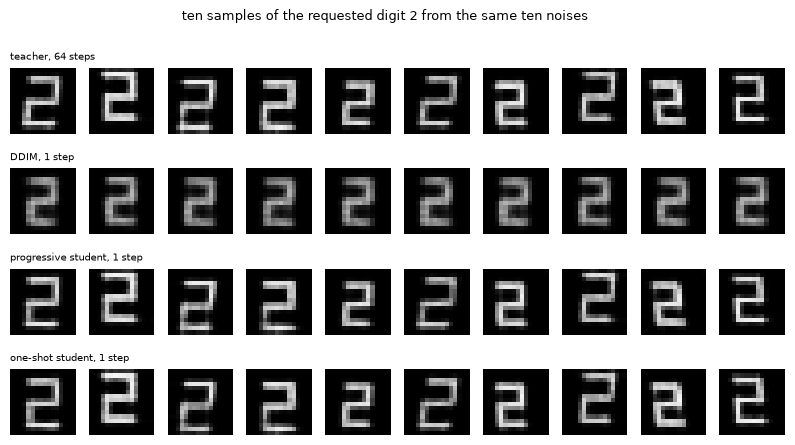
One-step DDIM produces the average glyph of each digit. It is recognizable, so validity stays at 0.993, but all variety is gone (style spread 0.0025, FID 226). The one-step student keeps the teacher’s variety at FID 6.3: 64× cheaper sampling for ~3 FID points. Six rounds took 43 s, against 29 s to train the teacher.
One-shot distillation for comparison. Luhman & Luhman (2021) proposed the obvious alternative: run the full teacher on many noises once, then regress a one-step student on the (noise → sample) pairs. With 20,000 pairs (1.3 M teacher evaluations; progressive used 1.5 M) and 6000 updates, the one-shot student reaches FID 4.10, valid 0.978 — slightly better than the progressive one. On this small problem, the teacher’s map from noise to latents is smooth enough to regress in one go, and the single regression avoids six rounds of accumulated error.
The paper’s argument for progressive distillation is about cost at scale. Its teachers use up to 8192 steps, so one training pair costs 8192 network evaluations, and a one-shot student starts far from its target map. Our experiment does not test that regime.
3.6 What the paper reports, and what came next
The paper distills models on CIFAR-10, ImageNet 64×64 and LSUN bedrooms and churches (128×128), starting from samplers with up to 8192 steps. It reports, for example, FID 3.0 on CIFAR-10 with 4 steps, and quality degrading gracefully down to 1–2 steps.
Limitations:
- the rounds are sequential;
- errors accumulate over rounds;
- a guided teacher needs extra care (Meng et al.’s guided distillation distills the guided prediction, with w as an input).
Later few-step methods remove the round structure: consistency models (Lecture 18) learn a map from any point of the ODE trajectory to its end; adversarial and distribution-matching distillation add a GAN-like loss (Lecture 10 §5).
4. simple diffusion (Hoogeboom, Heek & Salimans)
4.1 The problem
In 2022, high-resolution image diffusion took one of two detours:
- cascades — a 64 × 64 model followed by super-resolution diffusion models (Imagen, DALL·E 2);
- latent diffusion — diffuse in a compressed autoencoder space (Stable Diffusion; §5.1).
Both add components, training stages and failure modes. simple diffusion asks: what does it take to train one diffusion model directly on 256–512 px pixels and match them? Its answer is a short list of modifications; the most general one is about the noise schedule.
4.2 The noise schedule must depend on the resolution
Take a noisy image at resolution and average-pool it by a factor :
Averaging independent noise values divides their variance by . A natural image is smooth at the scale of a few pixels, so is essentially the same image at resolution . The pooled noisy image is therefore a low-resolution image at SNR times higher:
The global structure of an image lives in its low-resolution version. So at the same t, a 512-px image’s global structure is times less noisy than a 64-px image’s. With a schedule designed for 64 px, the 512-px model sees its composition destroyed only at the very end of the forward process. In the reverse direction, it must decide the composition in the first few steps and spends nearly all its time on details. The fix shifts the whole schedule toward noise:
For , every SNR is divided by 64. The paper also proposes an interpolated schedule — moving from the shifted schedule at high noise toward a less shifted one at low noise — to keep enough training at the levels that matter for fine detail. Chen (2023, §5.3) reaches the same conclusion from a different direction.
4.3 Experiment: the same glyph at three resolutions
Training pixel-space models at 32–64 px is beyond our CPU budget (Lecture 12 §5.3), so code 06 tests the claim on the forward process directly.
- Data. It renders the same 2000 glyphs at 16, 32 and 64 px: the same shapes, sampled more finely (
HiResGlyphWorld). - Noising. It noises them with the cosine schedule, with and without the shift (shift = d/16; our base resolution is 16, the paper’s 64).
- Measurement. It asks how often the exact Bayes classifier — the posterior over digits under an empirical prior of 5000 glyphs, applied after pooling to 16 px — still recognizes the digit:
| t | log-SNR | 16 px | 32 px | 32 px, shifted | 64 px | 64 px, shifted |
|---|---|---|---|---|---|---|
| 0.5 | 0.00 | 0.834 | 0.948 | 0.830 | 0.973 | 0.830 |
| 0.7 | −1.35 | 0.537 | 0.841 | 0.505 | 0.947 | 0.542 |
| 0.8 | −2.25 | 0.342 | 0.645 | 0.335 | 0.897 | 0.308 |
| 0.9 | −3.68 | 0.203 | 0.326 | 0.193 | 0.624 | 0.184 |
| 0.95 | −5.07 | 0.132 | 0.201 | 0.133 | 0.311 | 0.131 |
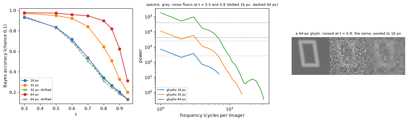
At t = 0.8 the digit is recognizable in a third of the 16-px glyphs and in 90% of the 64-px ones. With the unshifted schedule, a 64-px model must settle which digit within the first ~10% of the reverse process (accuracy is already 0.62 at t = 0.9); at 16 px the digit forms gradually between t ≈ 0.9 and 0.6. The shift puts all three resolutions back on the same curve, to within sampling noise.
4.4 The other ingredients
The paper’s remaining modifications are about where to spend compute in a U-Net at high resolution:
- Scale the low-resolution part. Put the extra blocks (and, in their U-ViT variant, transformer layers) at the 16 × 16 level, where global structure is computed and feature maps are cheap. Keep the high-resolution levels thin.
- Downsample early. Use an invertible downsampling in the first layer (a discrete wavelet transform or a patchify), so no full-resolution feature maps are needed.
- Dropout only at low resolution. Regularize where the capacity is.
- Multiscale loss. Add the loss evaluated on downsampled versions of the prediction, to weight the low frequencies — the global structure — more.
The paper reports that a single pixel-space model trained this way reaches FIDs on ImageNet 128–512 competitive with cascaded and latent models. It also reports that the same recipe works for text-to-image generation.
4.5 The spectral view: diffusion generates coarse structure first
The pooling argument has a frequency-domain twin (Dieleman, Diffusion is spectral autoregression). The power spectrum of natural images falls roughly as ; Gaussian noise has a flat spectrum. A noisy image’s spectrum is approximately signal plus a constant noise floor, and the floor rises with t. So the forward process drowns frequencies from the top down: fine detail disappears first, global layout last. The reverse process then restores them from the bottom up — an approximate autoregression over frequencies, coarse to fine.
Code 06, Part 2 computes the highest frequency (cycles per image) at which the mean signal power still exceeds the noise floor:
| t | glyphs 16 px | 32 px | 64 px | 64 px, shifted | dead leaves 64 px |
|---|---|---|---|---|---|
| 0.3 | 4 | 6 | 8 | 4 | 13 |
| 0.5 | 3 | 4 | 6 | 3 | 8 |
| 0.7 | 0 | 3 | 4 | 0 | 4 |
| 0.8 | 0 | 1 | 3 | 0 | 2 |
| 0.9 | 0 | 0 | 1 | 0 | 0 |
The dead leaves images of Lecture 2 have a power spectrum ∝ , close to natural images. Their cutoff descends smoothly from 13 cycles at t = 0.3 to 0 at t = 0.9: a coarse-to-fine schedule over frequencies. The glyphs at 64 px keep more cycles per image than at 16 px at every t, and the shifted schedule brings them back exactly onto the 16-px cutoffs. This is §4.3 in the frequency domain: a larger image has more signal power per frequency band relative to the per-pixel noise.
The view also explains Lecture 12’s “shared intermediate latents” (coarse content decided first) and why the schedule — how long the sampler spends at each cutoff — matters so much.
5. Optional readings
5.1 Latent diffusion (Rombach et al. 2022)
The division of labour. Most bits of an image are imperceptible high-frequency detail. Rombach et al. separate perceptual compression from semantic compression:
- an autoencoder (trained once with a perceptual and a patch-adversarial loss, and a light KL or VQ penalty — the VQ-GAN recipe of Lecture 9) maps images to a latent grid times smaller per side;
- the diffusion model only has to model the latent grid.
The paper reports that – gives the best trade-off: smaller factors leave the diffusion model too much work; larger ones lose detail in the autoencoder. Conditioning on text enters through cross-attention. Stable Diffusion is this design.
We have used this idea since Lecture 12 §5.3: a pixel-space MLP DDPM gave valid 0.44 on glyphs, the same algorithm on Lecture 8’s 64 latent numbers 0.90. Every glyph experiment of this lecture runs in that latent space. Latent diffusion and simple diffusion are two answers to the same question. One moves the problem to a space where it is small; the other keeps pixels and fixes the schedule and the architecture so that the model spends its effort where the information is.
5.2 EDM: the design space (Karras et al. 2022)
EDM rewrites every diffusion model in one form: (variance exploding; the VP form is the same after dividing by α, ). The model is a denoiser . Its probability-flow ODE is
EDM then treats the pieces as independent design choices.
Sampling as ODE solving.
- DDIM is Euler’s method on this ODE. Code 05, Part 1 checks it: DDIM in VP variables and Euler on EDM’s ODE agree to .
- Heun’s second-order method. Take an Euler step, re-evaluate the slope at the new point, and use the average. It costs 2 evaluations per step instead of 1 (except the last step).
- The time grid. with ρ = 7, which spends most steps at small σ, where trajectories bend.
- Optional stochasticity (“churn”): add a little noise and denoise again, as a corrector.
The paper reports CIFAR-10 FIDs of 1.79 (class-conditional) and 1.97 (unconditional) with 35 network evaluations.
Code 05 isolates the sampler from the network with an exact denoiser (the 8-mode ring is a Gaussian mixture), so every error is discretization error. Mean distance to the exact ODE solution from the same noise:
| NFE | Euler = DDIM, cosine grid | Euler, log-σ grid | Euler, ρ = 7 | Heun, cosine grid | Heun, ρ = 7 |
|---|---|---|---|---|---|
| 5 | 0.177 | 0.266 | 0.140 | 26.9 | 6.87 |
| 9 | 0.046 | 0.081 | 0.078 | 1.33 | 2.73 |
| 17 | 0.029 | 0.035 | 0.033 | 0.137 | 0.147 |
| 33 | 0.017 | 0.016 | 0.015 | 0.027 | 0.013 |
| 65 | 0.009 | 0.008 | 0.007 | 0.006 | 0.002 |
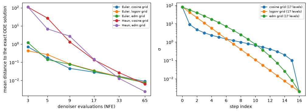
- At large budgets EDM’s choices win. Euler’s error falls roughly as 1/NFE, Heun’s much faster; at 65 NFE, Heun on the ρ = 7 grid is 3–4× more accurate than any Euler variant.
- At small budgets they lose. At ≤ 17 NFE, Heun is far worse than Euler: its corrector evaluates the slope after a huge step, where it means nothing. And no time grid wins at every budget. A better ODE solver does not give few-step generation; §3 and Lecture 18 do.
- The grid also changes the spread of the samples. The cosine grid ends with one large jump (σ = 0.2 → 0.002 in the 9-level grid). Its last step replaces x by , which is tighter than the data, so samples are pulled onto the mode centres (spread 0.03–0.04 instead of the data’s 0.05). This happens with the deterministic and the ancestral sampler alike — Lecture 8 §2.4’s tightening, from the sampler’s side.
Preconditioning. EDM writes the network as
with (unit-variance input), , (unit-variance target for ), loss weight , and the data’s standard deviation. These are chosen so that the network’s input and target both have unit variance at every σ, and so that ‘s errors are amplified as little as possible.
Translate to VP variables with (, ; Exercise 7):
- ;
- ;
- ;
- the loss weight is .
So is v-prediction () with v’s plain MSE. The parameterization question of §3.3 and code 03 is a preconditioning question:
- ε-prediction has , , which blows up at high noise;
- x-prediction has , so the network must reproduce its input at low noise;
- v (EDM with ) is bounded everywhere.
EDM also samples training noise levels from a log-normal around the levels that matter most. That is a schedule choice again.
5.3 Noise schedules and input scaling (Chen 2023)
Chen makes the same observation as simple diffusion — the optimal schedule depends on image size — from a different angle. Scaling the input by () shifts the log-SNR by . So “use a noisier schedule” and “scale the image down” are the same intervention. Chen proposes simple families of schedules (cosine, sigmoid) plus input scaling, and reports that with them a pixel-space model (the RIN architecture) trains well at high resolution in a single stage. Together with simple diffusion and Lecture 12 §5.4’s T = 500 result, the lesson is consistent: where on the log-SNR axis training happens matters more than how many steps the chain has.
5.4 unCLIP (Ramesh et al. 2022, “DALL·E 2”)
unCLIP generates in two stages through CLIP’s joint image–text embedding space:
- a prior maps a caption to a CLIP image embedding. The paper tries an autoregressive prior and a diffusion prior, and reports that the diffusion prior is comparable or better and cheaper;
- a decoder — a diffusion model, followed by two super-resolution diffusion models — generates the image from that embedding.
Because the decoder is conditioned on an image embedding, an existing image can be encoded and decoded again into variations that keep its semantics, and two images can be interpolated in embedding space. Classifier-free guidance is used in both stages. The paper reports greater diversity than GLIDE at similar photorealism in human evaluations. It is a cascade and a latent model at once: the “latent” is a semantic embedding rather than a compressed image.
5.5 Diffusion is spectral autoregression (Dieleman 2024)
This is §4.5. The blog’s measurement is the radially averaged power spectral density of natural images. On a log–log plot it is close to a straight line (a power law), and noise adds a horizontal floor that rises with the noise level. Its argument is that diffusion is approximately autoregression over frequencies — approximately, because the cutoff is soft and the same network handles all frequencies jointly. That is why the analogy to Lecture 5’s autoregression is a lens, not an identity. It also explains why schedules tuned for one image size (one spectrum) fail at another.
6. The big picture
6.1 Three fixes, one recurring theme
| question | answer of this session | what our experiments added |
|---|---|---|
| How to follow a condition more strongly? | CFG: , one network with label dropout | It corrects the gap between the data’s and what we want (noisy labels, weak models); with no gap, it only costs. It does not sample the tilted distribution, and deterministic samplers overshoot. |
| How to sample in a few steps? | Progressive distillation with v-prediction | 1 step at FID 6.3 vs the 64-step teacher’s 3.5. ε breaks at α → 0; x needs a skip connection. One-shot distillation was as good at our scale. |
| How to diffuse at high resolution? | Shift the schedule by ; spend capacity at 16 × 16 | Pooling shows the 2 log k effect directly; the shift realigns recognizability and spectral cutoffs across resolutions. |
The recurring theme is the noise-level axis:
- guidance acts mostly at high noise;
- distillation fails where α → 0;
- schedules decide how much time each frequency band gets;
- samplers decide where to put their steps.
Choosing what happens at each log-SNR is most of the craft of diffusion models.
6.2 How they combine in practice
A 2023–2024 text-to-image system typically has these parts:
- latent diffusion: an autoencoder with ;
- a v- or flow-matching parameterization (Lecture 16);
- a resolution-dependent schedule shift (Stable Diffusion 3 shifts its timesteps by resolution, Lecture 17);
- classifier-free guidance with a scale of 3–8;
- a solver with 20–50 steps, or a distilled few-step student (consistency or adversarial distillation, Lectures 10 and 18) when speed matters.
Each of the papers of this session supplied one of these parts.
7. Summary
- Notation. , log-SNR . ε-, x- and v-prediction are interchangeable given , but each implies a loss weighting (SNR, 1, SNR + 1) and divides by something different (α, σ, nothing).
- Classifier-free guidance. Bayes’ rule makes an implicit classifier gradient; one network with label dropout gives both. In 2-D, guidance trades diversity for class-likeness but overshoots beyond the class (57% outside at w = 8 with DDIM). On glyphs it was useless with clean labels (FID 3.7 → 117 by w = 4) and helpful with noisy labels (FID 8.2 → 2.9 at w = 0.5, on-class 0.68 → 0.89).
- Progressive distillation. Two teacher DDIM steps become one student step, and the rounds repeat. With v-prediction a 1-step student covers all 8 modes of the ring (DDIM: 0) and reaches FID 6.3 on glyphs (DDIM: 226). ε-prediction breaks as α → 0.
- simple diffusion. Pooling by k raises the effective log-SNR by 2 log k, so high-resolution models need a noisier schedule. At t = 0.8 the digit is recognizable in 34% of 16-px glyphs and in 90% of 64-px ones; the shift brings 64 px to 31%.
- EDM. DDIM = Euler; Heun with ρ = 7 is best at 33–65 NFE and worst at ≤ 17. Preconditioning with σ_d = 1 is v-prediction.
- Spectra. Noise drowns frequencies from the top down, so diffusion generates coarse structure first.
8. Common pitfalls
- “Guidance always improves samples.” It corrects a gap between the model’s conditional distribution and the one we want. With clean, non-overlapping classes and a good model, every w > 0 made FID worse (§2.5).
- “CFG samples .” It tilts each noisy marginal, which is not the same; deterministic guided samplers overshoot beyond the data (§2.4).
- “w and the guidance scale are the same number.” ; papers and libraries differ.
- “A better ODE solver makes one-step sampling possible.” One step from noise can only return the conditional mean; second-order solvers are worse than Euler at very few steps (§5.2). Few-step sampling needs a network trained for it (§3, Lecture 18).
- “ε-, x- and v-prediction are equivalent.” Mathematically interchangeable, numerically not: they weight the noise levels differently and amplify errors differently (§1.2, §3.4).
- “The schedule that works at 64 px works at 512 px.” The same t is far less noisy for a larger image; shift it by (§4.2).
- “Distillation is always cheaper than direct regression.” At our scale one-shot distillation was as good and as cheap; the advantage of progressive rounds is about expensive teachers (§3.5).
9. Exercises
Exercise 1 (the implicit classifier). Show , and that the CFG prediction corresponds to the score .
Answer
By Bayes, ; the last term does not depend on z. By Tweedie (Lecture 12 §7.2), and , where is the posterior mean of the noise. Subtract.
For the second part, gives the score . Equivalently, it is — classifier guidance with the implicit classifier.
Exercise 2 (guide in any parameterization). Show that guiding , or with the same w gives the same DDIM update.
Answer
For fixed z and t, each conversion in §1.2 is affine: e.g. . An affine map commutes with combinations whose weights sum to 1: , because the constant term appears with total weight . So guiding ε and then converting equals converting and then guiding x (or v). DDIM’s update is affine in , so the samplers agree.
Exercise 3 (parameterizations as weightings). Show and .
Answer
ε. and , so . Square it: the factor is .
v. and , so , i.e. . Finally, .
Consequence. ε-prediction gives the noisy levels (SNR → 0) almost no weight in x-space. v keeps weight ≥ 1 everywhere — “SNR + 1” in the paper’s table.
Exercise 4 (the distillation target). Derive in §3.2, and check that with (, ) it equals the teacher’s second .
Answer
One DDIM step from with prediction lands at . Setting this equal to and collecting gives .
At : , which is the teacher’s second step’s output, .
The denominator vanishes only if , i.e. , which never happens.
Exercise 5 (DDIM is Euler). Show that DDIM’s update, written for and , is Euler’s method for .
Answer
DDIM. Divide by :
Euler. .
These are the same, with . Code 05 checks it numerically to .
Exercise 6 (the shift). Derive the shift from average pooling. How large is it for 256 px relative to 64 px, in log-SNR and in SNR? What does simple diffusion’s rule do at d = 32?
Answer
Pooling by k divides the noise variance by and leaves a smooth signal unchanged, so the effective SNR of the low-resolution image is multiplied by : . To give a -px model the same coarse-scale corruption as a 64-px model at every t, subtract .
For d = 256: , i.e. every SNR is divided by 16.
At d = 32 the rule adds : a smaller image needs a less noisy schedule, by the same argument in reverse.
Exercise 7 (EDM preconditioning is v-prediction). With , and , show , , and .
Answer
. Hence:
- , so ;
- , so ;
- .
So , which is with . The weight is v’s plain MSE (Exercise 3).
Exercise 8 (why one deterministic step returns the mean). Show that the minimizer of is , and that as it tends to . Why does a distilled student escape this?
Answer
The minimizer. The minimizer of a squared error over functions of is the conditional mean.
The limit. As , carries no information about x, so . That is code 03’s one-step DDIM landing at the ring’s centre, and code 04’s average glyph.
Why the student escapes. Its training target is not x but , the end point of the teacher’s deterministic trajectory from . That is a function of , so there is no averaging over x. The student learns a map from noise to samples, as a GAN generator or a normalizing flow does.
Exercise 9 (hands-on).
(a) In 02_cfg_glyphs.py, sample the noisy-label model with the ancestral sampler (eta=1.0). Does the FID-optimal w change?
(b) In 03_distill_2d.py, give the x-prediction Denoiser a skip connection: output z + net(...) for small t. How close do you get to v?
(c) In 06_resolution_spectra.py, add 128 px (k = 8). Predict the accuracy at t = 0.9 before running.
Answer (sketch)
(a) In 2-D the ancestral sampler overshot much less (§2.4), so expect higher w to remain usable: the FID minimum should move to a larger w or become flatter.
(b) A skip with as removes the identity-learning problem. Choosing and output scale σ recovers v exactly (Exercise 7).
(c) The shift is in log-SNR. At t = 0.9 (λ = −3.68) the effective λ at 16 px is ≈ +0.48, between t = 0.3 and 0.5 on the 16-px curve, so expect an accuracy around 0.85–0.9.
10. Further reading
Required papers
- J. Ho, T. Salimans, Classifier-Free Diffusion Guidance, NeurIPS 2021 Workshop (arXiv 2207.12598).
- T. Salimans, J. Ho, Progressive Distillation for Fast Sampling of Diffusion Models, ICLR 2022.
- E. Hoogeboom, J. Heek, T. Salimans, simple diffusion: End-to-end diffusion for high resolution images, ICML 2023.
Optional papers of the session
- R. Rombach et al., High-Resolution Image Synthesis with Latent Diffusion Models, CVPR 2022.
- T. Karras, M. Aittala, T. Aila, S. Laine, Elucidating the Design Space of Diffusion-Based Generative Models, NeurIPS 2022.
- A. Ramesh et al., Hierarchical Text-Conditional Image Generation with CLIP Latents, 2022.
- T. Chen, On the Importance of Noise Scheduling for Diffusion Models, arXiv 2023.
- S. Dieleman, Diffusion is spectral autoregression (blog), 2024.
Background and follow-ups
- P. Dhariwal, A. Nichol, Diffusion Models Beat GANs on Image Synthesis, NeurIPS 2021 (classifier guidance).
- J. Song, C. Meng, S. Ermon, Denoising Diffusion Implicit Models, ICLR 2021 (DDIM).
- E. Luhman, T. Luhman, Knowledge Distillation in Iterative Generative Models for Improved Sampling Speed, 2021 (one-shot distillation).
- C. Meng et al., On Distillation of Guided Diffusion Models, CVPR 2023.
- D. Kingma et al., Variational Diffusion Models, NeurIPS 2021 (log-SNR notation).
- M. Chidambaram et al., What does guidance do? A fine-grained analysis in a simple setting, 2024; A. Bradley, P. Nakkiran, Classifier-Free Guidance is a Predictor-Corrector, 2024.
Related notes in this course
- Lecture 10 (truncation; Diffusion2GAN); Lecture 12 (DDPM, Tweedie, the VP-SDE); Lecture 8 §2.4 (few-step tightening); Lecture 2 (dead leaves and natural-image spectra).
11. Next lecture
Lecture 14: Diffusion without Gaussian denoising (reading session · 10/24).
This lecture treated Gaussian noise as given and tuned everything around it. Lecture 14 asks whether the noise is needed at all. Cold diffusion replaces it with deterministic degradations — blur, masking, pixelation — and still restores images step by step. Inverse heat dissipation uses the heat equation, which erases high frequencies first — the spectral view of §4.5, made literal. InDI turns restoration into small direct iterations, trading distortion for perceptual quality. A recurring question will be diversity: a deterministic degradation has a deterministic inverse, so where does the variety of samples come from?