Maps to: MIT 6.S978 Deep Generative Models (Fall 2024), Reading · Tue 11/05/2024 · Flow Matching 2 (student paper session). Required papers:
- P. Esser, S. Kulal, A. Blattmann, R. Entezari, J. Müller, H. Saini, Y. Levi, D. Lorenz, A. Sauer, F. Boesel, D. Podell, T. Dockhorn, Z. English, K. Lacey, A. Goodwin, Y. Marek, R. Rombach, Scaling Rectified Flow Transformers for High-Resolution Image Synthesis (Stable Diffusion 3), ICML 2024;
- N. Ma, M. Goldstein, M. S. Albergo, N. M. Boffi, E. Vanden-Eijnden, S. Xie, SiT: Exploring Flow and Diffusion-based Generative Models with Scalable Interpolant Transformers, ECCV 2024;
- I. Gat, T. Remez, N. Shaul, F. Kreuk, R. T. Q. Chen, G. Synnaeve, Y. Adi, Y. Lipman, Discrete Flow Matching, NeurIPS 2024.
Basis: This session consisted of student presentations, with no published slides. The notes take Lecture 16’s view that flow matching is one regression surrounded by separable design choices. The first two papers ask which choices matter when the model becomes large; the third carries the whole framework to tokens. Background the papers rely on (latent diffusion, DiT, classifier-free guidance for flows) comes first. Paper claims are labelled “the paper reports”. All experiments were designed for these notes and run on a CPU, on the glyph latents of Lecture 12 and the toy language of Lecture 15. They test the papers’ design axes at a size where nothing can be “scaled”. Several outcomes differed from what I expected or from the papers, and are reported as they came out:
- SD3’s preferred time sampler helped most at few steps, but not with an adaptive solver, and its second-best sampler failed on our small images;
- noise prediction did not just lose to velocity prediction — it broke the ODE sampler;
- the linear scheduler beat the paper’s quadratic one for discrete flow matching, and the corrector did not help on short sentences;
- our small MLP beat our small Transformers.
Code:
code/lecture17/— 4 scripts + the shared modulescaling_fm.py. They run in 75–115 s. Reading time: 4 hours including running the code.
0. How to read this lecture
0.1 Where we are
Lecture 16 built flow matching from three equivalent papers and isolated its design choices:
- the path (linear, cosine, VP);
- the target the network regresses (velocity, noise, data);
- the time distribution used in training;
- the sampler (ODE solver, or an SDE).
On a CPU, with 2-D mixtures and 64-number glyph latents, every choice could be checked against exact answers. This session’s papers ask the same questions where it matters commercially:
| paper | question | answer in one line |
|---|---|---|
| SD3 (Esser et al.) | which formulation and backbone for large text-to-image models? | rectified flow with logit-normal time sampling, a two-stream Transformer (MM-DiT), a resolution-dependent time shift; validation loss scales smoothly up to 8 B parameters |
| SiT (Ma et al.) | on a fixed DiT backbone, which design steps from DDPM to flow matching actually help? | continuous time, the linear or cosine interpolant, velocity prediction and an SDE sampler with a tuned diffusion coefficient: each a measurable gain |
| Discrete flow matching (Gat et al.) | can flow matching work on discrete tokens? | yes: probability paths per token, a “probability velocity” built from a denoiser; masked diffusion is one scheduler of it |
0.2 Learning goals
- Explain latent DiT and its conditioning (adaLN-Zero), and how SD3’s MM-DiT extends it to text (§1, §2.3).
- Explain why non-uniform time sampling helps and how it relates to loss weighting; derive SD3’s resolution shift as a log-SNR shift (§2.1–2.2).
- List SiT’s design steps and their measured effects. Derive the family of SDEs with the same marginals as the flow ODE, and explain the role of the diffusion coefficient (§3).
- Explain why noise prediction is fragile at the noise end, in flow-matching time (§3.3).
- Define discrete probability paths and velocities, derive the mask-path velocity, and relate it to masked diffusion. Explain schedulers and corrector sampling (§4).
0.3 Notation and time direction
These notes keep Lecture 16’s convention: t = 0 noise, t = 1 data, . The papers differ:
| paper | data at | noise at | their interpolant | in our notation |
|---|---|---|---|---|
| SD3 | t = 0 | t = 1 | our = their | |
| SiT | t = 0 | t = 1 | , | |
| Discrete FM | t = 1 | t = 0 (source) | same direction as ours |
Formulas quoted from SD3 and SiT are converted where they are used.
0.4 Map
| Section | Content | Code |
|---|---|---|
| §1 | Background: latent DiT, adaLN-Zero, guidance for flows | 03_dit_conditioning.py |
| §2 | Stable Diffusion 3: time sampling, resolution shift, MM-DiT, scaling | 01_time_sampling.py, 03_dit_conditioning.py |
| §3 | SiT: interpolant, target, ODE vs SDE | 02_sit_ablations.py |
| §4 | Discrete flow matching | 04_discrete_fm.py |
| §5 | The design space, summarized | — |
1. Background: the latent diffusion Transformer
1.1 Latent space and patches
Large image generators do not work on pixels. As in Lecture 13 §5.1 (latent diffusion), an autoencoder compresses an image into a latent grid: for SD3, 8× smaller per side with 16 channels. The generative model works on that grid. A diffusion Transformer (DiT; Peebles & Xie 2023) then:
- cuts the latent grid into patches, each one a token;
- adds position embeddings;
- runs Transformer blocks over the token sequence;
- maps each output token back to a patch of the velocity (or noise).
Our glyph latents (Lecture 12’s tokenizer) are already 16 tokens of 4 numbers: a 4 × 4 grid of patches. TinyDiT treats them exactly this way.
1.2 Feeding the condition: in-context, adaLN, adaLN-Zero
The network needs the time t and the condition (class, or text). DiT compared four ways and found one clearly best. Our TinyDiT implements three of them:
- In-context. Append the time and class embeddings as two extra tokens; plain Transformer blocks must find them by attention.
- adaLN (adaptive LayerNorm). Remove the LayerNorms’ own scale and shift parameters. Predict them from the condition vector = time embedding + class embedding: . Every token in every block is modulated by the condition. This is FiLM (P2) applied to Transformers.
- adaLN-Zero. adaLN plus a per-channel gate on each residual branch: . The layer that produces is initialized to zero, and so is the final output layer. Each block starts as the identity, and the whole network outputs 0.
Code 03, Part 1 confirms the initialization: adaLN-Zero’s output is exactly 0, and its first block changes its input by 0%. The adaLN and in-context blocks change theirs by 50% and 41%.
Part 2 trains each variant for 2000 steps (batch 64) on class-conditional flow matching, with Lecture 16’s MLP for reference:
| network | parameters | loss at step 750 / 1750 | FID (w = 0) | valid | on-class | train |
|---|---|---|---|---|---|---|
| DiT, adaLN-Zero | 247 k | 55.97 / 44.22 | 11.7 | 0.886 | 0.946 | 28 s |
| DiT, adaLN | 222 k | 57.54 / 44.92 | 14.2 | 0.865 | 0.922 | 27 s |
| DiT, in-context | 165 k | 58.70 / 46.22 | 16.7 | 0.832 | 0.895 | 30 s |
| MLP (VelocityNet 512 × 3) | 1.98 M | 53.76 / 40.22 | 6.2 | 0.975 | 0.985 | 7 s |
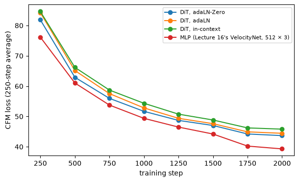
- DiT’s ordering reproduces: adaLN-Zero < adaLN < in-context, in loss at every checkpoint and in sample quality. Modulation acts on every token in every block at no extra sequence length.
- The MLP wins here. It has 8× the parameters and is 4× faster per step on a CPU. A Transformer pays off when the number of tokens and the model grow — SD3’s regime, not 16 tokens and 2000 steps. Do not read the course’s toy results as an argument against Transformers at scale.
The paper reports DiT-XL/2 (675 M parameters, 2 × 2 patches) at FID 2.27 on class-conditional ImageNet 256 with guidance. It also reports FID improving steadily with the Transformer’s compute (Gflops), whether that comes from model size or from smaller patches.
1.3 Classifier-free guidance for flows
A flow model is trained with label dropout like a diffusion model (Lecture 13 §2.3). Guidance extrapolates the velocity:
The velocity is affine in the score for a fixed (Lecture 16 §3.2), so this is the same guidance as on ε or the score. In code 03, w = 1 puts 99.9% of the adaLN-Zero model’s samples on the requested digit (from 94.6%) and raises validity (0.89 → 0.95). FID worsens (11.7 → 20.4) because the labels are clean and guidance removes style variety — exactly Lecture 13’s finding. SD3 samples with guidance throughout.
2. Stable Diffusion 3 (Esser et al.)
2.1 Which times to train on
The question. Rectified flow’s loss averages over . But not all times are equally hard:
- Near the noise end the optimal velocity is nearly : easy (Lecture 16 Exercise 6).
- Near the data end almost determines : easy again.
- In the middle the network must decide which image is forming: hard. That is where its errors concentrate (Lecture 16 §2.3 measured the loss floor and the model’s error per t).
SD3 therefore samples t from a density that favours the middle. Sampling t from π is the same as uniform sampling with the loss multiplied by π(t) (Exercise 4), so the choice of π is a choice of loss weighting. The paper compares, in its own time direction:
- logit-normal: , . A bump in the middle; m moves it toward data () or noise ().
- mode sampling with heavy tails: , . is uniform; larger s favours the middle, while the ends keep some weight.
- CosMap: , the density of the cosine schedule.
The paper reports a study of 61 formulations (rectified flow, ε- and v-prediction, EDM, LDM schedules, and the time samplers above). Each was trained on ImageNet and CC12M and ranked by non-dominated sorting of CLIP score and FID over 24 settings (sampler steps, EMA, dataset). Rectified flow with logit-normal(0, 1) had the best average rank (1.54), and was first at 5 sampling steps (1.25). Rectified flow with uniform time sampling did not beat the LDM baseline; only rectified-flow variants with modified time sampling did.
Code 01 compares the samplers on glyph latents: same network and budget (2500 steps), a second seed of the uniform baseline to measure run-to-run noise, and three sampling settings. First, the densities, as the share of draws in each range of our t:
| sampler | [0, 0.1) | [0.1, 0.3) | [0.3, 0.7) | [0.7, 0.9) | [0.9, 1] |
|---|---|---|---|---|---|
| uniform | 0.100 | 0.200 | 0.400 | 0.201 | 0.100 |
| logit-normal(0, 1) | 0.014 | 0.184 | 0.603 | 0.185 | 0.014 |
| logit-normal(1, 0.6) | 0.023 | 0.578 | 0.399 | 0.001 | 0.000 |
| mode, s = 1.29 | 0.047 | 0.124 | 0.660 | 0.123 | 0.047 |
| CosMap | 0.071 | 0.188 | 0.484 | 0.188 | 0.070 |
The resulting mini FIDs:
| sampler | Euler, 5 steps | Euler, 25 steps | dopri5 (~40 NFE) | valid (dopri5) |
|---|---|---|---|---|
| uniform | 76.7 | 23.5 | 15.0 | 0.879 |
| uniform, second seed | 78.2 | 23.3 | 13.8 | 0.877 |
| logit-normal(0, 1) | 59.9 | 22.3 | 17.6 | 0.909 |
| logit-normal(1, 0.6) | 77.8 | 51.2 | 46.6 | 0.688 |
| mode, s = 1.29 | 65.5 | 20.1 | 14.1 | 0.908 |
| CosMap | 69.9 | 20.8 | 12.3 | 0.894 |
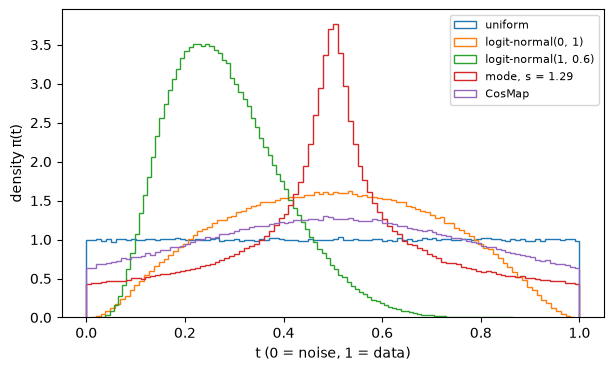
- The noise level of the comparison is the gap between the two uniform seeds: 1.5, 0.1 and 1.2 FID.
- At few steps, favouring the middle helps clearly. With 5 Euler steps all three middle-favouring samplers beat uniform by 8–18 FID, logit-normal most. That is the regime where SD3 reports its clearest win.
- With an accurate solver, the ranking changes. CosMap is best (12.3) and logit-normal(0, 1) worst of the middle samplers (17.6). The logit-normal draws only 1.4% of its times beyond t = 0.9, so the last details near the data are learned less well, although its valid rate is the highest. No single sampler wins every column. The mode and CosMap samplers, which keep some weight at the ends, are good throughout.
- SD3’s runner-up fails here. Logit-normal(1, 0.6), second in the paper’s ranking, almost never trains near the data and reaches only FID 47. SD3 trains on 256² and larger images, where a given t destroys less of the image, so shifting training toward noise helps them. Our 64-number glyphs are the opposite case — the subject of §2.2.
2.2 The resolution shift
Lecture 13 §4 showed, with simple diffusion, that the same noise level destroys less of a larger image: average pooling by k raises the effective log-SNR by . So high-resolution models need noisier schedules. SD3 makes the same argument for rectified flow. A constant image of n pixels, noised to time t, has posterior uncertainty about its value . Matching that uncertainty between resolutions n and m gives (in SD3’s time, 1 = noise)
This is exactly a log-SNR shift. For rectified flow, . Substituting gives , so (Exercise 2). Code 01, Part 3 checks it to round-off:
| α | = 0.25 → | 0.5 → | 0.75 → | |
|---|---|---|---|---|
| 1 | 0.250 | 0.500 | 0.750 | 0 |
| 2 | 0.400 | 0.667 | 0.857 | 1.386 |
| 3 | 0.500 | 0.750 | 0.900 | 2.197 |
With for pixel counts, : simple diffusion’s rule. The paper reports choosing for 1024² images by a human preference study, with a strong preference for shifts above 1.5. It applies the shift in both training and sampling.
2.3 MM-DiT and scaling
Two modalities, two streams. A text-to-image model must condition on a whole sentence, not one label. SD3 uses three text encoders:
- two CLIP models, whose pooled embeddings feed the adaLN modulation together with the time embedding;
- T5-XXL, whose token sequence enters the Transformer.
Earlier models fed text tokens through cross-attention. SD3’s MM-DiT instead:
- concatenates text tokens and image tokens into one sequence for joint attention: every image token can attend to every word, and every word to every image patch;
- gives each modality its own weights: separate QKV projections, MLPs and modulation parameters. The two kinds of tokens live in different spaces and only meet in attention.
It is in-context conditioning (§1.2) with separate parameters for the conditioning stream, plus adaLN-Zero modulation by the pooled text and the time.
Stabilization. At large scale, attention logits grew until training diverged in mixed precision. SD3 normalizes queries and keys with RMSNorm (QK-normalization) in both streams.
Scaling. The paper reports:
- Validation loss falls smoothly with model size and training steps, with no sign of saturation, from depth 15 to depth 38 (8 B parameters).
- Validation loss predicts the other metrics: GenEval, human preference and T2I-CompBench.
- Text and typography improve with T5. Removing T5 at sampling time keeps aesthetics (50% win rate against the full model) but hurts typography (38%).
- The largest model (depth 38, with DPO fine-tuning) scores 0.74 on GenEval at 1024², against 0.67 for DALL·E 3.
Our code 03 is the smallest possible version of this backbone. It reproduces DiT’s ordering of conditioning methods, and shows that at 16 tokens an MLP is the better choice. The scaling claims cannot be tested on a CPU.
3. SiT: one design choice at a time (Ma et al.)
3.1 The ladder from DiT to SiT
SiT keeps DiT’s backbone and walks from DDPM to an interpolant model in steps, measuring each. The paper reports, for SiT-B at 400 k iterations (FID-50K, 250 function evaluations):
| step | setting | FID |
|---|---|---|
| DiT-B (discrete-time DDPM, noise prediction) | 44.2 | |
| continuous time | VP path, score prediction | 43.6 |
| + loss weighting | VP, weighted score | 39.1 |
| velocity prediction | VP, velocity | 39.8 |
| change the interpolant | Linear, velocity | 34.8 |
| GVP (= our cosine path), velocity | 34.6 | |
| SDE sampler | Linear, velocity, | 33.6 |
| GVP, velocity, | 32.9 |
The largest single gain is the interpolant. At XL size with guidance (cfg 1.5), the paper reports FID 2.15 with the ODE and 2.06 with the SDE, against DiT-XL’s 2.27.
3.2 An SDE for every diffusion coefficient
The probability-flow ODE is not the only way to move to . For any ,
has the same marginals (Exercise 1: the extra drift cancels the extra diffusion in the Fokker–Planck equation). The score comes from the velocity model by Lecture 16 §3.2’s conversion, so one trained network drives a whole family of samplers.
- is the ODE.
- Larger injects fresh noise and lets the score term pull samples back toward high density. This corrects accumulated errors, at the price of needing more steps.
SiT compares, in our time direction:
- (their ; it vanishes at the data end);
- (vanishes at both ends);
- , which minimizes a KL bound and equals β for the VP path. It is infinite at the noise end; our code caps it at 10.
The paper reports that the best depends on both the interpolant and the prediction.
3.3 Our ablation
Code 02 trains four models — {linear, cosine} × {velocity, noise} — with the same network and budget. It samples each with the ODE and with the SDE (mini FID / valid; every sampler starts at ):
| model | ODE Euler, 50 | ODE Heun, 25 (50 NFE) | SDE , 50 | SDE , 250 | SDE , 250 | SDE , 250 |
|---|---|---|---|---|---|---|
| linear, velocity | 19.1 / 0.88 | 15.3 / 0.88 | 21.6 / 0.91 | 17.2 / 0.90 | 14.2 / 0.90 | 15.3 / 0.91 |
| linear, noise | 460 / 0.10 | 498 / 0.02 | 450 / 0.14 | 186 / 0.45 | 195 / 0.45 | 65 / 0.67 |
| cosine, velocity | 19.1 / 0.84 | 18.9 / 0.85 | 22.0 / 0.86 | 21.5 / 0.85 | 18.9 / 0.85 | 21.7 / 0.89 |
| cosine, noise | 321 / 0.08 | 347 / 0.03 | 325 / 0.12 | 139 / 0.47 | 152 / 0.44 | 58 / 0.70 |
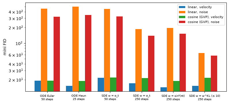
Prediction target: noise prediction breaks the ODE. SiT reports velocity prediction ahead of noise/score prediction by a few FID. Here the gap is catastrophic. Part 2 of the script shows why:
| t | RMS error of | RMS error of | |
|---|---|---|---|
| 0.001 | 0.068 | 1000 | 68.2 |
| 0.01 | 0.067 | 100 | 6.6 |
| 0.1 | 0.110 | 10 | 0.99 |
| 0.5 | 0.383 | 2 | 0.38 |
Near the noise end the noise is easy to name (error 0.07), but turning it into a velocity requires , which divides by . At every error is multiplied by 1000. This is Lecture 13 §3.3’s argument against ε-prediction for one-step students, here breaking an ordinary ODE sampler. Diffusion models avoid it by not starting at exact pure noise (), and their samplers by working with and together (DDIM).
The SDE samplers partly rescue the noise models (FID 65 and 58 with ): their score term never divides by , and the injected noise washes out early mistakes.
Interpolant. With velocity prediction, the linear path did somewhat better than the cosine path here (Heun 15.3 vs 18.9); SiT found them equal (34.8 vs 34.6). Lecture 16 §2.5 showed that the two define the same exact flow, so the difference lies in learning. The velocity loss weights the noise levels differently on the two paths (Lecture 16 Exercise 4).
Sampler. For the linear velocity model:
- at 50 network calls the ODE wins (Heun 15.3; SDE 21.6);
- with 250 steps the SDE catches up and slightly passes it (: 14.2; : 15.3 with the best valid rate, 0.91);
- the best differs between models.
All three points agree with SiT, which samples its SDE with 250 steps and reports a gain of 0.1 FID over the ODE at XL size.
4. Discrete flow matching (Gat et al.)
4.1 Probability paths over tokens
For a sequence of tokens from a vocabulary, a continuous velocity makes no sense. Gat et al. move probability mass instead. The source can be all-[MASK] sequences or uniform random tokens; the target is the data. Per token, a conditional path mixes the two ends with a scheduler (, ):
With the mask source this is Lecture 15’s absorbing process run forwards in our time: each token has been revealed with probability . The sequence path factorizes over tokens given , and the marginal path mixes over the data, as in Lecture 16 §2.1.
4.2 Probability velocities
A probability velocity gives, for token i in the current sequence z, the rate at which probability flows from to each other value. It must have non-negative off-diagonal entries and sum to zero. One Euler step samples every token independently:
As in the continuous case, a velocity generates a path if it satisfies the discrete continuity (Kolmogorov) equation, and marginal velocities are posterior averages of conditional ones. For the convex path the paper derives
where is the probability denoiser: the posterior of the clean token given the current sequence. It is learned with a cross-entropy loss on the clean tokens.
With the mask source, does not depend on t (the paper’s Proposition 3.1; Lecture 15 §4.1 found the same for SEDD and RADD). Lecture 15’s masked-diffusion network is such a denoiser, and one trained network serves every scheduler.
What the formula means for sampling: in a step of size h, a [MASK] token is revealed with probability , its value drawn from the denoiser; a revealed token stays. With that probability is , exactly masked diffusion’s in Lecture 15’s reversed time (Exercise 7).
Code 04, Part 1 checks this with one trained denoiser (Lecture 15’s TokenNet, cross-entropy on masked tokens, 3000 steps, 41 s):
| sampler | grammatical | −log p_data | distinct |
|---|---|---|---|
| Lecture 15 masked diffusion, 12 steps | 0.510 | 0.914 | 1980 |
| discrete FM, κ = t, 12 steps | 0.515 | 0.923 | 1972 |
| Lecture 15 masked diffusion, 64 steps | 0.781 | 0.915 | 1954 |
| discrete FM, κ = t, 64 steps | 0.767 | 0.904 | 1955 |
They agree within sampling noise (±0.01–0.02 with 2000 samples). Discrete flow matching with the mask path contains masked diffusion as one scheduler.
4.3 Schedulers
The scheduler decides when tokens are revealed. The paper parameterizes a cubic family of schedulers and, for text, picks by generative perplexity. Code 04, Part 2 samples the same denoiser with three schedulers (fraction grammatical):
| κ_t | 6 calls | 12 calls | 24 calls | 64 calls |
|---|---|---|---|---|
| t (linear) | 0.308 | 0.507 | 0.661 | 0.780 |
| t² | 0.259 | 0.480 | 0.674 | 0.773 |
| t³ | 0.172 | 0.420 | 0.637 | 0.764 |
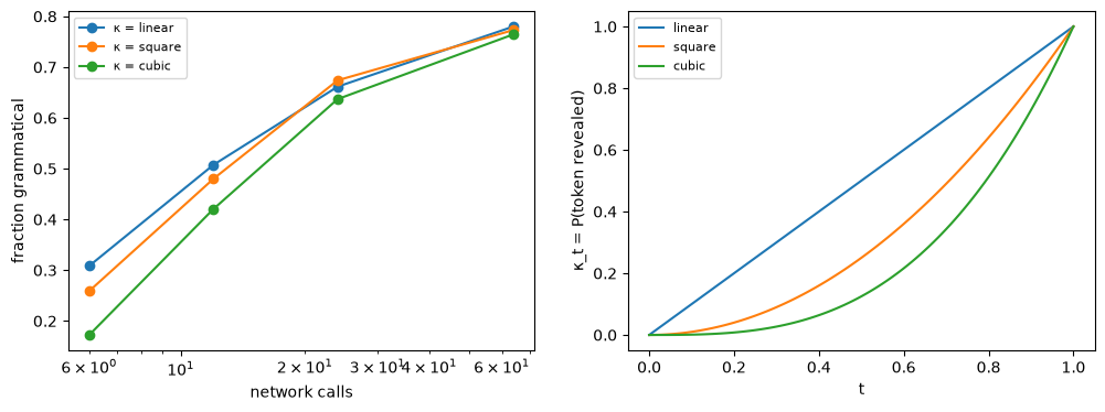
I expected the convex schedulers to win: they reveal few tokens early, when choices are made with little context. They lose instead, most clearly at few calls. The expected number of tokens revealed in a step is (Exercise 8):
- for it is constant, ;
- for and it grows toward the end, so the last steps reveal many tokens together.
Tokens revealed together are drawn independently (Lecture 15 §5), and late collisions are as damaging as early ones. The paper’s choice of comes from 1024-token texts scored by an external model’s perplexity. On a 12-word grammar it does not carry over.
4.4 Corrector sampling
The velocity can be combined with a backward velocity that moves probability back toward the source:
With the mask source, re-masks revealed tokens at rate . The combination still generates the same path, so the sampler can revise early choices. The paper uses and reports a significant improvement in generation quality. Code 04, Part 3, with :
| corrector c | 24 calls: grammatical | 64 calls: grammatical |
|---|---|---|
| 0 (off) | 0.648 | 0.764 |
| 1 | 0.627 | 0.777 |
| 3 | 0.616 | 0.771 |
| 10 | 0.463 | 0.759 |
- With 64 calls all settings are within sampling noise.
- With 24 calls re-masking hurts (strongly at c = 10). Every re-masked token must be revealed again, so a small budget is spent on churn.
A 12-word sentence leaves little to revise; the paper’s gains are for long texts at hundreds of calls.
4.5 What the paper reports
- Text. With 150 M-parameter models (Llama-2 generative perplexity at 256 / 512 / 1024 function evaluations), the mask path gives 34.2 / 30.0 / 22.5 and the mixture path with uniform noise 30.0 / 27.5 / 22.3. Campbell et al.’s discrete flows give 38.5 / 33.5 / 28.7.
- Code, 1.7 B parameters. HumanEval pass@1 6.7% against 14.3% for an autoregressive model of the same size and data; MBPP 6.7% against 17.0%. With the answer’s length given, 11.6% and 13.1%.
- Images. CIFAR-10 FID 3.63 at 1024 evaluations, generating discrete pixels.
Discrete flow matching narrowed the gap to autoregression without closing it. This is the same picture as Lecture 15’s masked diffusion vs AR on our toy language.
5. The design space, summarized
| axis | options | what our experiments showed | what the papers chose |
|---|---|---|---|
| path | linear, cosine (GVP), VP | same exact flow (L16 §2.5); linear easiest to integrate and learn here | SD3, SiT: linear (SiT also GVP) |
| target | velocity, noise, data, score | noise prediction breaks samplers near pure noise (§3.3) | velocity (SD3, SiT) |
| time sampling | uniform, logit-normal, mode, CosMap | middle-favouring helps at few steps; ends matter for accurate solvers (§2.1) | logit-normal(0, 1) (SD3) |
| resolution | shift of t / log-SNR | = simple diffusion’s shift (§2.2) | α = 3 at 1024² (SD3) |
| backbone | MLP, U-Net, DiT, MM-DiT | adaLN-Zero best among DiT variants; MLP best at 16 tokens (§1.2) | MM-DiT (SD3), DiT (SiT) |
| sampler | ODE (Euler, Heun, adaptive), SDE with | SDE ≈ ODE at 5× the steps (§3.3) | Euler 28–50 steps (SD3); SDE 250 steps (SiT) |
| tokens | mask path, κ_t, corrector | κ = t best on short sentences; corrector neutral (§4) | κ = t², corrector (DFM) |
A pattern runs through the table. Each choice moves effort to where the problem is hardest:
- time sampling: to the middle of the path;
- the shift: to higher noise for larger images;
- velocity prediction: away from divisions by small numbers;
- the SDE: into correcting errors;
- the scheduler: toward an even spread of decisions.
Whether a choice helps depends on where the difficulty lies in a given problem. Several of the papers’ preferences did not transfer to our small one, for identifiable reasons.
6. Summary
- Latent DiT. Latent patches are tokens. adaLN-Zero conditions every block through gated modulation and starts each block as the identity. On our glyph latents: adaLN-Zero FID 11.7 < adaLN 14.2 < in-context 16.7. At 16 tokens an MLP is better (6.2).
- SD3, time sampling. Favouring the middle of the path helps most at few steps (5 Euler steps: FID 60 vs 77 for uniform). With an accurate solver the ends matter again, and the samplers with heavy tails (mode, CosMap) were best overall.
- SD3, resolution shift. is the log-SNR shift , simple diffusion’s rule.
- MM-DiT. Two streams with separate weights and joint attention; QK-norm for stability. The paper reports smooth scaling up to 8 B parameters, with validation loss predicting human preference.
- SiT. Interpolant (largest gain), velocity prediction, SDE sampling with a model-dependent . Any gives the same marginals. Noise prediction is fragile at the pure-noise end (×1000 error at t = 0.001).
- Discrete flow matching. Probability paths and velocities on tokens. The mask-path velocity is ; κ = t is masked diffusion. On short sentences the linear scheduler won and the corrector did not help.
7. Common pitfalls
- “Logit-normal time sampling is always better.” It helps where the middle of the path is the bottleneck, at few sampling steps. It starves the ends, which an accurate solver needs (§2.1).
- “Shift toward noise for better samples.” The shift compensates for resolution. Small images need less noise, and logit-normal(1, 0.6) failed on ours (§2.1–2.2).
- “Noise prediction and velocity prediction are interchangeable.” Mathematically yes. Numerically, recovering from divides by (§3.3).
- “The SDE sampler is better than the ODE.” Only with enough steps and a suitable ; at 50 steps the ODE won (§3.3).
- “adaLN-Zero is a regularizer.” It is an initialization: each block starts as the identity and grows through its gate (§1.2, Exercise 5).
- “Discrete flow matching is a new model.” With the mask source and κ = t it is masked diffusion. What it adds is the framework: schedulers, other sources, correctors (§4).
- Copying formulas across time conventions. SD3 and SiT put data at t = 0, discrete flow matching and these notes at t = 1 (§0.3).
8. Exercises
Exercise 1 (one family of SDEs). Show that has the same marginals as , given that v generates .
Answer
The Fokker–Planck equation of the SDE is
Since , the middle term is , which cancels the last one. What remains, , is the continuity equation that v satisfies (Lecture 16 §1.2). So solves both equations from the same start. The noise spreads the density out; the score term pulls it back by exactly as much.
Exercise 2 (the resolution shift). Show that SD3’s satisfies for rectified flow, (SD3’s time).
Answer
.
Divide by : .
Take : . Every SNR is divided by , the ratio of pixel counts — Lecture 13 §4.2’s pooling argument.
Exercise 3 (SiT’s ). In our time direction . Evaluate it for the linear path, and show that it equals for the VP path.
Answer
Linear path (, ):
It is infinite at the noise end and 0 at the data end.
VP path. and . Then and . So
and : the VP-SDE’s own diffusion coefficient. With it, the SDE above is the reverse-time diffusion of Lecture 12.
Exercise 4 (time sampling = loss weighting). Show that training with has the same expected gradient as training with and the per-time loss multiplied by .
Answer
, and gradients pass through expectations.
The two estimators have the same mean but different variances. Sampling the important times more often is importance sampling, and is usually less noisy than up-weighting rare ones. SD3 writes the equivalent weight in its ε-loss form as .
Exercise 5 (adaLN-Zero at step 0). At initialization, which parameters of an adaLN-Zero block receive a nonzero gradient?
Answer
The block computes , with because the modulation layer is zero.
- The branch’s own parameters (attention, MLP): zero gradient, because their output is multiplied by .
- γ and β: zero gradient for the same reason.
- The gate α: nonzero gradient, . Through α, the modulation layer’s weights get a gradient.
In addition, the network’s final layer is also zero, so at step 0 only that final layer receives a gradient at all. The network “opens” from the output inward: first the final layer, then the gates, then the branches. Every intermediate state is a sensible function, never a random deep network.
Exercise 6 (the mask path’s velocity generates it). For one token with the mask source, show that under the probability of still being masked at time t is .
Answer
A masked token leaves the mask state at rate (the velocity’s total off-diagonal mass, since sums to 1 over real tokens); revealed tokens never return.
With : and . The solution is , since then ✓. The revealed value is drawn from the denoiser, so the revealed tokens have the right conditional distribution.
Exercise 7 (κ = t is masked diffusion). Show that one Euler step of discrete flow matching with reveals a masked token with the same probability as Lecture 15’s masked-diffusion sampler.
Answer
Discrete flow matching. From t to t + h, a masked token is revealed with probability .
Lecture 15. Lecture 15’s time is (the masking probability). Going from τ to , its sampler reveals with probability .
Both draw the revealed value from the same denoiser. Code 04, Part 1 confirms the equivalence statistically.
Exercise 8 (where the reveals happen). For and N uniform steps, how many of the L tokens are revealed, in expectation, in the last step? Evaluate for L = 12, N = 6 and p = 1, 2, 3.
Answer
: the last step takes κ from to 1. With L = 12 and N = 6:
- p = 1: 2 tokens;
- p = 2: 12(1 − 25/36) ≈ 3.7;
- p = 3: 12(1 − 125/216) ≈ 5.1.
The convex schedulers reveal almost half the sentence in one final step, all drawn independently. This is why they did worst at 6 calls (code 04: 0.31, 0.26, 0.17).
Exercise 9 (hands-on).
(a) In 01_time_sampling.py, train with a mixture: 90% logit-normal(0, 1) and 10% uniform. Does it keep the 5-step gain and lose the dopri5 penalty?
(b) In 02_sit_ablations.py, sample the noise model with DDIM-style updates, i.e. the posterior-mean step , instead of the velocity. Does the catastrophe disappear?
(c) In 04_discrete_fm.py, use a confidence-based order (MaskGIT, Lecture 7): at each step reveal the masked tokens whose denoiser is most confident. Compare with κ = t at 6 and 12 calls.
Answer (sketch)
(a) Expect most of the 5-step gain to remain (the middle is still sampled heavily). The 10% uniform share restores training near both ends, which should remove most of the dopri5 penalty: a “heavy tails” design like the mode sampler’s.
(b) The posterior-mean update uses , which still divides by in the first steps. The big error then appears in the very first state rather than through the velocity. Starting at a larger helps, and clipping (as DDPM implementations clip ) helps more.
(c) Confidence ordering avoids revealing ambiguous tokens together, so expect a clear gain at few calls. The paper notes, though, that it biases the distribution: diversity (the distinct count) should drop.
9. Further reading
Required papers
- P. Esser et al., Scaling Rectified Flow Transformers for High-Resolution Image Synthesis, ICML 2024.
- N. Ma et al., SiT: Exploring Flow and Diffusion-based Generative Models with Scalable Interpolant Transformers, ECCV 2024.
- I. Gat et al., Discrete Flow Matching, NeurIPS 2024.
Background and follow-ups
- W. Peebles, S. Xie, Scalable Diffusion Models with Transformers (DiT), ICCV 2023.
- R. Rombach et al., High-Resolution Image Synthesis with Latent Diffusion Models, CVPR 2022.
- A. Campbell, J. Yim, R. Barzilay, T. Rainforth, T. Jaakkola, Generative Flows on Discrete State-Spaces, ICML 2024 (discrete flow models on CTMCs).
- M. S. Albergo, N. M. Boffi, E. Vanden-Eijnden, Stochastic Interpolants: A Unifying Framework for Flows and Diffusions, 2023 (the SDE family of §3.2).
- Black Forest Labs, FLUX.1 (2024), a rectified-flow Transformer in SD3’s lineage. Movie Gen (Lecture 19) uses flow matching for video.
Related notes in this course
- Lecture 16 (flow matching, paths, velocity–score conversion); Lecture 13 (guidance, parameterizations, the resolution shift); Lecture 15 (masked diffusion, SEDD); Lecture 7 (MaskGIT’s confidence ordering); P2 (FiLM, Transformer blocks).
10. Next lecture
Lecture 18: Consistency models (guest lecture by Yang Song · 11/21).
Every sampler in Lectures 12–17 integrates an ODE or SDE step by step, and quality saturates only after dozens of network calls. Lecture 16’s reflow and distillation reached one step by straightening the flow or regressing its end points. Consistency models take another route: learn a function that maps any point of an ODE trajectory directly to its end, enforced by self-consistency between neighbouring points. It can be trained from a pretrained model (distillation) or from scratch (consistency training). We will reuse Lecture 16’s glyph flow model as a teacher.