Maps to: MIT 6.S978 Deep Generative Models (Fall 2024), Reading · Tue 10/08/2024 · GAN 1 (student paper session). Required papers:
- A. Sauer, T. Karras, S. Laine, A. Geiger, T. Aila, StyleGAN-T: Unlocking the Power of GANs for Fast Large-Scale Text-to-Image Synthesis, ICML 2023;
- M. Kang, J.-Y. Zhu, R. Zhang, J. Park, E. Shechtman, S. Paris, T. Park, Scaling up GANs for Text-to-Image Synthesis (GigaGAN), CVPR 2023;
- M. Kang, R. Zhang, C. Barnes, S. Paris, S. Kwak, J. Park, E. Shechtman, J.-Y. Zhu, T. Park, Distilling Diffusion Models into Conditional GANs (Diffusion2GAN), ECCV 2024.
Optional: Z. Tu, Learning Generative Models via Discriminative Approaches, CVPR 2007.
Basis: This session consisted of student presentations, with no published slides. The notes are organized around the session’s question: “after diffusion models took over text-to-image generation, can GANs — with their one-pass sampling — be scaled up, or at least serve as fast students of diffusion models?” Numbers from the papers are labelled “the paper reports” and given only where the claim is central. The StyleGAN background the papers build on (StyleGAN 1–2) is explained first. All experiments were designed for these notes and run on a CPU:
- Tu’s classifier-boosting on a 2-D grid, where densities are exact;
- a caption-conditional style-based generator on glyphs, with style mixing and truncation;
- Diffusion2GAN’s recipe on a 2-D mixture, with an exact ODE teacher.
Results that differed from my plan are reported as they came out (e.g. our style mixing did not split “shape vs appearance” where I expected). Code:
code/lecture10/— 3 scripts + the shared modulescaling_gans.py. They run in 30–90 s. Reading time: 3–4 hours including running the code.
0. How to read this lecture
0.1 Where we are
Lecture 9 built GANs and met their problems: mode collapse, oscillation, sensitivity to losses and settings. Meanwhile, from 2021 on, diffusion models (Lectures 12–13) took over text-to-image generation: DALL·E 2, Imagen, Stable Diffusion. They train stably, cover the data distribution well, and follow complex prompts. Their weakness is speed: tens to hundreds of network evaluations per image.
GANs have the opposite profile. They generate in one forward pass, and their latent spaces support editing (interpolation, style mixing), but they had only been shown to work on narrow domains (faces, cars) or class-conditional ImageNet. This session asks three questions:
- StyleGAN-T: can a GAN be made into a competitive text-to-image model, by changing its architecture, its discriminator and its conditioning?
- GigaGAN: what breaks when a StyleGAN is scaled to a billion parameters and billions of images, and how is it fixed?
- Diffusion2GAN: if diffusion models are the best teachers, can a GAN be the best student, distilling a multi-step diffusion model into one step?
The optional 2007 paper by Zhuowen Tu is a precursor of the GAN idea: a generative model learned with a sequence of discriminative classifiers.
0.2 Learning goals
- Explain Tu’s discriminative generative learning (GDL), why it cannot collapse, and why it is expensive in high dimensions.
- Describe the StyleGAN generator: mapping network, style modulation (AdaIN, then weight (de)modulation), constant input, noise inputs, style mixing, truncation; and the R1 regularizer.
- Explain StyleGAN-T’s changes for text-to-image: text conditioning through the mapping network, a discriminator on frozen pretrained features, CLIP guidance, and the alignment vs variation trade-off.
- Explain GigaGAN’s additions: sample-adaptive kernel selection, attention layers, multi-scale training and discrimination, a separate upsampler.
- Explain Diffusion2GAN: distillation as paired translation from noise to image, regression + conditional adversarial loss, and why the adversarial term is needed.
- Compare GANs and diffusion models on speed, quality, diversity and control.
0.3 Map
| Section | Content | Code |
|---|---|---|
| §1 | Tu 2007: generative learning with classifiers | 01_discriminative_learning.py |
| §2 | The StyleGAN generator | 02_style_generator.py |
| §3 | StyleGAN-T | 02_style_generator.py |
| §4 | GigaGAN | — |
| §5 | Diffusion2GAN | 03_distill_ode.py |
| §6 | The big picture | — |
0.4 Data and metrics
- 2-D (scripts 01, 03): Gaussian mixtures on a circle of radius 2 (8 modes; std 0.2 in script 01, 0.05 in script 03). “Quality” is the fraction of samples within 3 std of a mode.
- Glyphs (script 02): captioned with Lecture 8’s three words — digit, slant (left / upright / right), thickness (thin / bold).
- The Judge reads the digit. Lecture 8’s pixel probe reads slant and thickness; on real glyphs it gets them right 96% / 89% of the time, which is the ceiling for “prompt following”.
- Real glyphs: valid 0.989, FID 0.60 on the 2000 test glyphs.
1. Tu 2007: a generative model from discriminative classifiers
1.1 The idea
Seven years before GANs, Zhuowen Tu asked how discriminative classifiers, which were then far better developed than generative models, could be used to learn a generative model.
Start with a simple model . At round t:
- Draw “negatives” from the current model and “positives” from the data.
- Train a classifier to separate them, with equal priors.
- Update
Why it works. With equal priors, Bayes’ rule gives — Lecture 9’s optimal discriminator, written as odds. With a perfect classifier one round gives . With a limited classifier each round removes what that classifier can see, and the rounds add up: a boosting of discriminative models into a generative one.
The catch. The model is a product , known only up to a normalizing constant. Drawing the next round’s negatives requires MCMC (Tu used Gibbs sampling), which is slow in high dimensions.
The GAN replaces “reweight the density, then sample it with MCMC” by “move the samples of a generator network along the classifier’s gradient”. Sampling becomes one pass, but the guarantees of reweighting are lost.
1.2 Experiment: boosting toward a ring
Code 01 stores the density on a 141 × 141 grid, so reweighting, normalizing and sampling are exact. The data are 8 Gaussians of std 0.2 on a circle, , and each round uses 2000 samples per class:
| classifier | KL(p_data ‖ p_t), rounds 0 → 1 → 2 → 3 … 8 | accuracy, round 1 → 8 | modes covered |
|---|---|---|---|
| weak (width 8) | 1.820 → 0.347 → 0.150 → 0.146 … 0.076 | 0.86 → 0.55 | 8 |
| medium (width 32) | 1.820 → 0.123 → 0.070 → 0.059 … 0.039 | 0.89 → 0.57 | 8 |
| strong (width 128) | 1.820 → 0.202 → 0.073 → 0.066 … 0.069 | 0.89 → 0.57 | 8 |
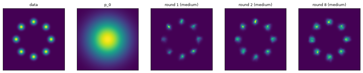
- One round removes most of the gap. Later rounds refine it until the classifier can no longer tell model from data (~0.55 accuracy on its own training samples).
- All 8 modes are covered from round 1 on. The model is reweighted, never moved, and is positive everywhere, so no mode can be lost.
- A stronger classifier is not better. It fits the noise of its finite training sample. The remaining error is estimation noise, and more samples per round reduce it: final KL 0.181 / 0.039 / 0.015 for 500 / 2000 / 8000 samples.
On the same data a non-saturating GAN (Lecture 9) covered all 8 modes in two seeds, with quality 0.97 and 0.88. These modes are four times wider than Lecture 9’s ring, where the same GAN collapsed. The structural difference stands: reweighting cannot lose a mode, moving samples can.
2. The StyleGAN generator
All three main papers build on the StyleGAN family (Karras et al. 2019, 2020, 2021; Sauer et al. 2022 for StyleGAN-XL). Its generator differs from Lecture 9’s “noise in, image out” network in five ways.
2.1 The ingredients
- Mapping network. An MLP (8 layers in StyleGAN) maps z to an intermediate latent w. The prior p(z) is fixed (Gaussian), but the distribution of w is learned, so w can be “unwarped”: directions in w space correspond more cleanly to factors of variation than directions in z.
- A learned constant input. The synthesis network starts from a learned 4×4 tensor, not from z.
- Style modulation. Every layer receives w through its own affine map , giving a style .
- StyleGAN 1 used AdaIN: normalize each feature map, then scale and shift it by the style.
- StyleGAN 2 moved the style into the weights. Modulation scales input channel i of the convolution weights by : . Demodulation rescales each output channel to unit norm: . This keeps the statistical effect of AdaIN and removes its characteristic “droplet” artifacts.
- Noise inputs. Per-pixel Gaussian noise, scaled by learned per-layer weights, is added after each layer. It models stochastic detail (hair strands, pores) so that w does not have to.
- Per-layer styles. Because every layer has its own style input, different layers can receive different w’s:
- Style mixing (coarse layers from , fine layers from ) shows what each resolution controls. In faces: pose and shape at coarse layers, colours and micro-structure at fine layers.
- The truncation trick pulls w toward the average style, . Smaller ψ gives more typical, higher-quality samples and less variety.
Regularization. StyleGAN2’s discriminator is trained with the R1 penalty , applied “lazily” every few steps. It smooths D around real data, and Lecture 11 shows why it makes GAN training locally convergent. A path-length regularizer encourages a smooth w → image map.
2.2 Experiment: a style-based generator at CPU scale
Code 02 builds TokenStyleG, a caption-conditional style generator for glyphs.
- Mapping: (z, sum of the caption’s word embeddings) → MLP → w. This is StyleGAN-T’s way of conditioning (§3).
- Synthesis: from a learned constant on a 2×2 grid of tokens (coarse), upsampled to 4×4 tokens (fine), each finally decoded into a 4×4 pixel patch. Every layer mixes tokens (spatial) and applies a modulated, demodulated linear map to channels, plus a noise input.
- Why tokens: a convolutional StyleGAN does the same with feature maps; tokens are ~10× cheaper on our CPU.
- Training: the discriminator is a small CNN with projection conditioning, . The loss is non-saturating, with lazy R1, Adam β = (0, 0.99), 3000 steps.
The comparison: a “plain” generator of the same size where the condition enters only at the input.
| generator | valid | FID | digit followed | slant followed | thickness followed | train |
|---|---|---|---|---|---|---|
| plain | 0.658 | 34.2 | 0.942 | 0.893 | 0.698 | 34 s |
| style-based | 0.807 | 44.4 | 0.982 | 0.936 | 0.795 | 50 s |
| real glyphs (rulers’ accuracy) | 0.989 | 0.60 | 1.000 | 0.963 | 0.894 |
- Both follow the caption. Lecture 9’s MLP GAN collapsed without conditioning; here the caption pins down the digit, and the style generator shows the asked digit 98% of the time.
- The style-based generator aligns better with the caption (every word) and makes more valid glyphs, while the plain one has the lower FID. Injecting the condition into every layer helps alignment, not automatically distribution matching.
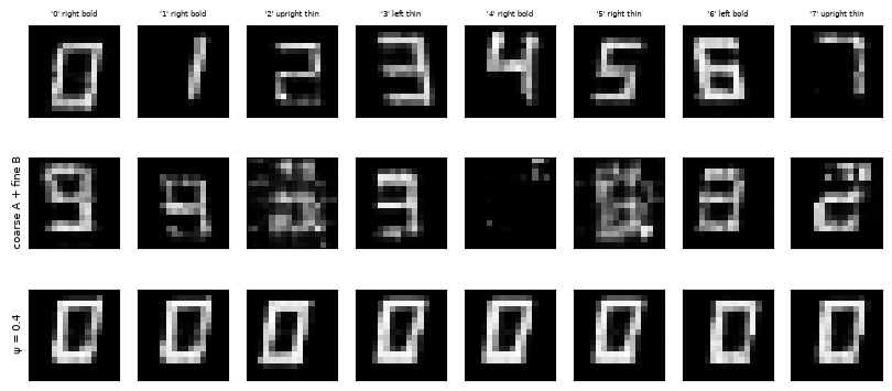
Style mixing (coarse layers styled by caption A, the rest by caption B; 1000 pairs that differ in all three words). Each cell gives the fraction of samples reading like A / like B:
| styles | digit: A / B | slant: A / B | thickness: A / B |
|---|---|---|---|
| all from A | 0.98 / 0.00 | 0.94 / 0.03 | 0.82 / 0.18 |
| coarse A + fine B | 0.06 / 0.61 | 0.16 / 0.67 | 0.36 / 0.64 |
| coarse B + fine A | 0.62 / 0.04 | 0.66 / 0.17 | 0.66 / 0.34 |
| all but the pixel layer A, pixel layer B | 0.67 / 0.05 | 0.80 / 0.10 | 0.42 / 0.58 |
I expected “coarse = digit, fine = thickness”. In our two-resolution generator it is not so: the 4×4 token layers decide the digit and slant as much as the 2×2 layers do. The clean split is the last layer. Styling only the pixel decoder with B transfers B’s thickness while keeping A’s digit and slant. Appearance lives in the last layer, shape in the earlier ones — StyleGAN’s coarse / middle / fine styles, with only two token resolutions to divide them.
Truncation toward each caption’s average style :
| ψ | valid | FID | digit followed | slant followed | thickness followed | diversity |
|---|---|---|---|---|---|---|
| 1.0 | 0.828 | 42.2 | 0.983 | 0.950 | 0.824 | 0.229 |
| 0.7 | 0.862 | 40.4 | 0.994 | 0.966 | 0.834 | 0.205 |
| 0.4 | 0.869 | 49.1 | 0.988 | 0.978 | 0.859 | 0.159 |
| 0.0 | 0.831 | 67.8 | 0.975 | 0.985 | 0.870 | 0.003 |
(Real glyphs sharing a caption: diversity 0.273.) Smaller ψ gives more typical glyphs that follow the words more closely, at the cost of diversity. At ψ = 0 every sample of a caption is the same glyph. The FID is best at a mild truncation and worst with none left. This is the GAN version of the trade-off that diffusion models control with the guidance scale (Lecture 13).
3. StyleGAN-T
3.1 Motivation
By 2022, the fastest text-to-image models were distilled diffusion models, still needing several network evaluations, while GANs had not been shown to handle open-ended text. StyleGAN-T asks what a GAN needs for large-scale text-to-image generation, with speed as the goal. The paper reports that it outperforms distilled diffusion models — the previous state of the art for fast text-to-image synthesis — in both sample quality and speed. Its advantage is clearest at low resolution; at higher resolutions the best (slow) diffusion models remain better.
3.2 What changes
Starting from StyleGAN-XL:
- Generator. The paper drops translation equivariance (StyleGAN3’s design goal, inherited by StyleGAN-XL) as unnecessary for this task, makes the convolutions residual, and increases capacity.
- Text conditioning. A pretrained CLIP text encoder embeds the prompt. The global text embedding is fed with z into the mapping network, so text acts through the styles of every layer. Code 02 does exactly this with its three word embeddings.
- Discriminator. Following Projected GANs, it is built on a frozen pretrained feature network (a self-supervised ViT, DINO). Lightweight trainable heads look at token features from several of its layers. Text enters through projection, and differentiable data augmentation is used. Strong pretrained features give the discriminator a good notion of “realistic” from the start, which speeds up and stabilizes training.
- CLIP guidance. An extra generator loss raises the CLIP similarity between the generated image and the prompt — a learned critic of alignment, beside the discriminator’s critic of realism.
3.3 Alignment vs variation
Text-to-image models must trade text alignment (does the image show what the prompt says?) against variation (do different samples differ?):
- diffusion models control this with the classifier-free guidance scale (Lecture 13);
- StyleGAN-T controls it with the truncation ψ and the strength of CLIP guidance.
The paper also describes a second training phase that adapts the text-encoder side with stronger CLIP guidance, improving alignment at the cost of variation. Code 02’s truncation table shows the same trade on a small scale: following the words improves while diversity falls.
4. GigaGAN
4.1 Motivation
GigaGAN asks whether GANs can be scaled like diffusion models and language models: a billion parameters, billions of images (LAION). The paper first reports that simply enlarging StyleGAN2 is unstable. Its architecture changes are what make scaling work.
4.2 Method
- Sample-adaptive kernel selection. A convolution layer holds a bank of N filters. For each sample, the style (from w and the text) computes softmax weights over the bank, and the layer uses their weighted average, which is then modulated and demodulated as in StyleGAN2. Capacity grows with N, but each sample uses one effective kernel. This is “more parameters without more compute per sample”, in the spirit of mixture-of-experts.
- Attention. Self-attention layers are interleaved with the convolutions for global structure, and cross-attention layers let image features attend to the individual text tokens, not just a global text embedding. For stability the paper uses L2-distance attention logits, which keep the layers better conditioned (Lipschitz) than dot products.
- Multi-scale training. The generator outputs an image pyramid (e.g. 64 down to 4 pixels). The discriminator judges every scale and checks consistency across scales, so coarse structure gets direct gradients.
- Discriminator losses. Besides real/fake, a matching-aware term treats real images with the wrong text as fakes, so D must check text alignment. A CLIP-based contrastive loss and a vision-aided loss from pretrained features are added.
- A separate upsampler. A second text-conditioned GAN upsamples the generated images to high resolution (applied repeatedly, up to 4K). It can also upsample the outputs of diffusion models.
4.3 What it reports
From the abstract:
- speed: about 0.13 s for a 512×512 image;
- resolution: 16-megapixel images in 3.66 s with the upsampler;
- editing: the latent space supports interpolation, style mixing and vector arithmetic, which diffusion models lack in this simple form.
Its zero-shot MS COCO FID is competitive with diffusion models of the time (Stable Diffusion v1.5, DALL·E 2), though not better than the best.
5. Diffusion2GAN: GANs as students of diffusion models
5.1 Distillation as paired translation
A diffusion model’s deterministic sampler (the probability-flow ODE, Lectures 12–13) defines a map Φ from a noise z to an image x. It is deterministic, but each evaluation needs many network passes.
Diffusion2GAN collects pairs (z, Φ(z)) by running the teacher’s ODE, and trains a one-step generator . It frames this as paired image-to-image translation (noise → image), the setting of pix2pix (Lecture 9 §6):
- Regression loss. The paper’s E-LatentLPIPS is a perceptual distance computed directly in the diffusion model’s latent space, with augmentations, so pairs can be compared without decoding to pixels.
- Conditional adversarial loss. The discriminator is built from the teacher diffusion model itself and conditioned on the text, at multiple scales.
It reports a one-step generator that outperforms contemporary one-step distillation methods on zero-shot COCO.
Why the adversarial term, if regression already has an exact target for every z? Code 03 shows why.
5.2 Experiment: distilling an exact ODE in 2-D
Code 03 uses 8 Gaussians of std 0.05 on a ring. For a Gaussian mixture, the noisy density at every diffusion level is again a Gaussian mixture, so the score is known in closed form and the teacher ODE is exact (gmm_eps, ddim_ode).
The teacher needs many steps even with a perfect score:
| ODE steps | 1 | 2 | 4 | 8 | 16 | 256 |
|---|---|---|---|---|---|---|
| quality | 0.000 | 0.001 | 0.549 | 0.952 | 0.999 | 0.993 |
With one step, every sample lands at , the data mean — the centre of the ring. Big steps cut across curved trajectories.
One-step students trained on 50,000 teacher pairs (two seeds):
| student | modes | quality | error vs teacher | quality, z near a boundary | quality, elsewhere |
|---|---|---|---|---|---|
| regression only | 8 / 8 | 0.858 / 0.887 | 0.080 / 0.075 | 0.42 / 0.44 | 0.924 / 0.955 |
| regression + adversarial, λ = 0.1 | 8 / 8 | 0.920 / 0.910 | 0.068 / 0.075 | 0.56 / 0.56 | 0.973 / 0.963 |
| regression + adversarial, λ = 1 | 8 / 8 | 0.924 / 0.924 | 0.079 / 0.083 | 0.57 / 0.55 | 0.978 / 0.980 |
| adversarial only (plain GAN) | 6 / 6 | 0.916 / 0.918 | 2.514 / 2.579 | — | — |
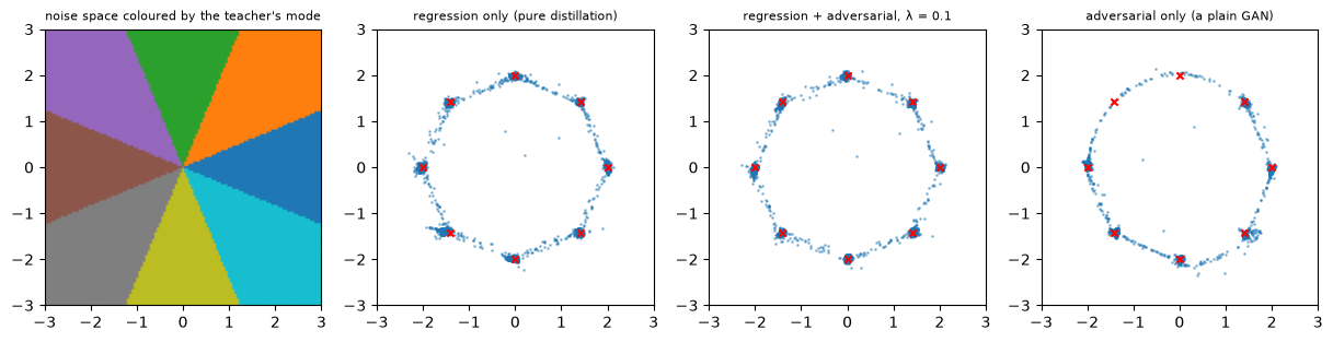
- Regression mostly works, because the target is deterministic: there is no averaging over several answers. The exception is where the map jumps. The ODE partitions noise space into 8 wedge-shaped regions, one per mode, and a smooth network cannot jump at their borders, so it lands between modes. For the 523 of 4000 test noises lying near a border, quality is 0.43; elsewhere it is 0.94.
- The adversarial term pushes border samples onto a mode (0.56) and tightens all the others (0.97–0.98), while keeping the pairing with the teacher (the error vs teacher is unchanged). This is Diffusion2GAN’s division of labour: regression keeps the student faithful to the teacher’s map and keeps training stable; the adversary removes the blur.
- A plain GAN without the teacher has to discover the modes by itself. It found 6 of 8 in both seeds (Lecture 9’s collapse) and kept no correspondence with the teacher’s map.
In images, “between modes” means a blurry average of two plausible images, and the borders are everywhere: every detail that could go two ways. That is why one-step students trained only by regression are blurry, and why an adversarial (or distribution-matching) term is part of every strong one-step distillation method.
6. The big picture
6.1 GANs vs diffusion models after this session
| GAN (StyleGAN-T / GigaGAN) | diffusion (Lectures 12–13) | |
|---|---|---|
| network passes per sample | 1 | 10s–100s (fewer with distillation) |
| training | adversarial; needs regularization (R1), pretrained-feature discriminators, careful architecture | regression; stable |
| coverage / diversity | weaker (collapse risk); truncation trades it away | strong |
| text alignment | CLIP guidance, matching-aware D, truncation | classifier-free guidance |
| latent space | w space: interpolation, style mixing, editing | noise → image map via the ODE; editing is harder |
| scale reported | ~1B parameters (GigaGAN) | larger |
6.2 Three ways a discriminator helps build a generator
| role of the classifier / discriminator | how the model changes | |
|---|---|---|
| Tu 2007 | its odds estimate p_data / p_model | the density is reweighted |
| GAN (StyleGAN-T, GigaGAN) | its gradient says “more real here” | the generator’s samples move |
| Diffusion2GAN | sharpens a regression to a teacher | a student imitates a slow model, minus its blur |
6.3 Where this goes
- Lecture 11 asks why GAN training is so fragile and what fixes it in principle: R1/R2 penalties and convergence, noise added to both distributions, and a link between GAN gradients and score functions.
- Lecture 13 returns to distillation from the diffusion side (progressive distillation). Lecture 18 covers consistency models, which reach one-step generation without an adversary.
7. Summary
- Tu 2007: a sequence of “data vs model” classifiers, each multiplying the model density by its odds, boosts a simple model toward the data. It cannot lose modes, but needs MCMC to sample in high dimensions. On a 2-D grid it cut KL from 1.82 to 0.04 in 8 rounds, limited by sample noise.
- StyleGAN’s generator: mapping network → w, learned constant, per-layer modulated / demodulated weights, noise inputs; per-layer styles allow style mixing, and truncation trades diversity for typicality. Our caption-conditional token version followed the words better than a plain generator. Truncation traded diversity for alignment as expected, and the last layer alone carried “appearance” (thickness).
- StyleGAN-T: text through the mapping network, a discriminator on frozen self-supervised features, CLIP guidance; fast text-to-image, best at low resolution.
- GigaGAN: adaptive kernel banks, self- and cross-attention, multi-scale generation and discrimination, matching-aware losses, an upsampler; ~1B parameters, 0.13 s per 512px image, an editable latent space.
- Diffusion2GAN: distill the teacher’s ODE map with regression plus a conditional adversarial loss. In 2-D, regression alone failed exactly at the borders where the map jumps; the adversarial term fixed part of that and sharpened the rest, while a plain GAN lost modes.
8. Common pitfalls
- “GANs are obsolete.” They remain the fastest generators and the strongest students of diffusion models (§5), and their adversarial losses train today’s tokenizers (Lecture 9).
- “Regression distillation is enough because the teacher is deterministic.” The teacher’s map has discontinuities (borders between outcomes); smooth regression blurs across them (§5.2).
- “Style mixing always separates coarse shape from fine appearance.” What each layer controls is learned and depends on the architecture (§2.2).
- “Truncation improves quality.” It improves typicality and alignment and lowers diversity; distribution metrics (FID) get worse beyond a mild setting (§2.2).
- “A stronger classifier always helps.” In Tu’s procedure, and in GAN discriminators, an over-fitting classifier injects noise (§1.2).
- “A discriminator on pretrained features is free.” It inherits what those features notice and ignore. And FID, computed with similar features, can be flattered by it — a caveat raised in later work on FID.
9. Exercises
Exercise 1 (Tu’s update). Show that if is the Bayes-optimal classifier for data vs with equal priors, the update gives after normalization. What does an update with a logistic-regression classifier (logit linear in features φ(x)) do to an exponential-family model ?
Answer
Optimal classifier. , so the odds are and , already normalized.
Logistic classifier. With logit , the update multiplies by , so and the model stays in the exponential family. Repeated rounds move θ until no linear classifier in φ can separate model from data. At that point : moment matching, the maximum-likelihood condition for exponential families. Tu’s procedure with linear classifiers is a form of maximum-entropy model fitting.
Exercise 2 (demodulation). For a linear layer with weights W (out × in) and style scales s (per input channel), show that if the inputs have i.i.d. unit-variance entries, the demodulated output has unit variance per output channel. Why is this preferable to AdaIN’s normalization of the activations?
Answer
Unit variance. The output is with . With independent unit-variance , . Dividing by makes this 1.
Why better than AdaIN. Demodulation normalizes based on the expected statistics implied by the weights, not on the actual activations of the sample. AdaIN normalizes each feature map by its measured mean and variance. The generator can then “smuggle” information past the normalization by creating a strong local spike (StyleGAN 1’s droplet artifacts) that dominates the statistics. Demodulation removes that incentive.
Exercise 3 (truncation and the mean). Why truncate toward the mean in w space rather than in z space? What changes when the truncation centre is the per-caption mean rather than a global mean?
Answer
w vs z. z ~ N(0, I) has its density peak at 0, but the generator’s notion of a “typical” sample lives in w space, after the mapping network has warped the distribution. Averaging in w gives an “average-looking” sample; averaging z would not, because the mapping is nonlinear.
Per-caption centre. A global mean would pull every sample toward an average of all captions — an unreadable blend of digits — and destroy alignment. Truncating toward keeps the condition and only reduces the within-caption variation. Code 02’s table shows alignment improving, not degrading, as ψ falls.
Exercise 4 (why one-step regression blurs). The teacher map Φ jumps across a border between two regions of noise space with outputs near and . A smooth student with Lipschitz constant K must move between and over a distance ≥ in z. Estimate the fraction of “in-between” samples, and explain how an adversarial term changes the optimum.
Answer
Fraction in between. Inside a band of width ~ around the border, G must pass through intermediate values. The fraction of in-between samples is roughly the Gaussian mass of the bands around all borders: proportional to the total border length times the band width. Larger mode separations (or lower capacity, smaller K) mean more blur. Code 03 found that the 13% of test noises near a border (within ±3°) produced most of the failures.
With an adversary. The regression loss alone is minimized by a smooth compromise. The adversarial term penalizes outputs where is small, so the optimum steepens the transition — pushes G toward a step — at a small regression cost on a thin band. With unlimited capacity both losses agree (G = Φ), so the adversary changes only what happens under limited capacity.
Exercise 5 (GigaGAN’s kernel selection). A layer has a bank of N kernels , and a sample with style w uses . Compare its parameters and compute cost with (a) one kernel N times wider, (b) a mixture of experts that runs all N kernels and mixes the outputs.
Answer
Parameters. N kernels, the same as (b) and the same order as (a).
Compute. One weighted sum of N kernels (cheap, independent of image size), then one convolution with the effective kernel. That is the cost of a single-kernel layer.
- (a) A wider layer would multiply the convolution cost by N.
- (b) Running all experts would also multiply it by N.
Because convolution is linear in the kernel, mixing kernels is equivalent to mixing outputs, so kernel selection gets mixture-of-experts capacity at single-kernel cost. The price is that the mixing weights are per sample, not per pixel.
Exercise 6 (hands-on).
(a) In 01_discriminative_learning.py, replace the MLP classifier by logistic regression on the features (x, y, x², y², xy). What does the model converge to?
(b) In 02_style_generator.py, add a third token resolution (1×1 → 2×2 → 4×4). Does style mixing separate more cleanly?
(c) In 03_distill_ode.py, train the regression student with 4× more parameters. How much of the border problem remains?
Answer (sketch)
(a) The model stays a Gaussian, , and converges to the Gaussian with the data’s mean and covariance (moment matching, Exercise 1) — a wide blob over the ring. Expressive classifiers are what make the method a good density estimator.
(b) A 1×1 stage can carry only global information (which digit, overall slant), so expect cleaner “shape vs appearance” splits. It is not guaranteed: what each layer encodes is learned.
(c) A larger student can make steeper transitions, so the border bands shrink and border quality rises. But any continuous G still has some in-between band, so the fraction should fall without reaching zero.
10. Further reading
The required and optional papers
- A. Sauer et al., StyleGAN-T: Unlocking the Power of GANs for Fast Large-Scale Text-to-Image Synthesis, ICML 2023.
- M. Kang et al., Scaling up GANs for Text-to-Image Synthesis (GigaGAN), CVPR 2023.
- M. Kang et al., Distilling Diffusion Models into Conditional GANs (Diffusion2GAN), ECCV 2024.
- Z. Tu, Learning Generative Models via Discriminative Approaches, CVPR 2007.
The StyleGAN family and its tools
- T. Karras, S. Laine, T. Aila, A Style-Based Generator Architecture for Generative Adversarial Networks, CVPR 2019.
- T. Karras et al., Analyzing and Improving the Image Quality of StyleGAN (StyleGAN2), CVPR 2020.
- A. Sauer, K. Chitta, J. Müller, A. Geiger, Projected GANs Converge Faster, NeurIPS 2021; A. Sauer, K. Schwarz, A. Geiger, StyleGAN-XL, SIGGRAPH 2022.
- T. Miyato, M. Koyama, cGANs with Projection Discriminator, ICLR 2018.
- L. Mescheder, A. Geiger, S. Nowozin, Which Training Methods for GANs do actually Converge?, ICML 2018 (R1; Lecture 11).
- T. Kynkäänniemi et al., The Role of ImageNet Classes in Fréchet Inception Distance, ICLR 2023 (the FID caveat of pitfall 6).
Related notes in this course
- Lecture 9 (GAN basics, the optimal discriminator as a density ratio, adversarial losses).
- Lecture 8 §1 (diffusion in one page; captions and the probe).
11. Next lecture
Lecture 11: Modern GAN theory — convergence, noise and scores (reading session · 10/10).
This lecture’s GANs worked because of a pile of stabilizers: R1 penalties, pretrained-feature discriminators, careful architectures. Lecture 11 asks what is actually wrong with the GAN game and what the minimal fix is:
- R3GAN derives a well-behaved loss (relativistic, with R1 and R2 penalties) and shows that, with it, a modern architecture needs none of the old tricks;
- Diffusion-GAN adds diffusion noise to both real and fake samples so that the two distributions overlap and the discriminator’s gradients mean something (Lecture 9’s JS problem);
- GANs Settle Scores! shows that the optimal GAN generator moves samples along the difference of score functions — the bridge from GANs to score matching and diffusion (Lecture 12).