Maps to: MIT 6.S978 Deep Generative Models (Fall 2024), Reading · Tue 09/10/2024 · Modeling Image Prior (student paper-presentation session). Required papers:
- D. Zoran & Y. Weiss, From Learning Models of Natural Image Patches to Whole Image Restoration (EPLL), ICCV 2011;
- D. Zoran & Y. Weiss, Natural Images, Gaussian Mixtures and Dead Leaves, NeurIPS 2012;
- D. Ulyanov, A. Vedaldi & V. Lempitsky, Deep Image Prior, CVPR 2018.
Optional:
- A. A. Efros & T. K. Leung, Texture Synthesis by Non-parametric Sampling, ICCV 1999;
- C. Barnes et al., PatchMatch, SIGGRAPH 2009;
- W. T. Freeman, T. R. Jones & E. C. Pasztor, Example-Based Super-Resolution, IEEE CG&A 2002.
Basis: In the original course this session consisted of student presentations, with no published slides. This lecture is organized around the three required papers themselves:
- the question they jointly answer (“what makes an image natural? what does a prior do in restoration?”) and the background it needs;
- each paper in turn: motivation, method, key experiments and limitations. Numbers taken from the papers are labelled “the paper reports”.
The optional papers are introduced briefly in §5. All experiments were designed for these notes. We download no natural-image dataset; instead, images generated by the “dead leaves model” stand in for natural images. This happens to be the very model the second paper uses to explain why GMMs work. Several results of the toy experiments disagree with the papers; all are reported faithfully in the text and in the code README. Code:
code/lecture02/(6 scripts + the shared moduleimage_priors.py; script 03 takes ~1.5 minutes the first time, script 06 ~80 seconds, the rest a few seconds) Reading time: 4–5 hours including running the code
0. How to read this lecture
0.1 What question these papers answer
Lecture 1 said that the core difficulty of generative modeling is “representing a distribution”. This lecture looks back more than a decade. Before anyone could generate high-resolution images, computer-vision researchers were already seriously answering a narrower but equally fundamental question:
What makes an image “natural”? That is: what does the distribution of natural images (the image prior) look like?
They cared mainly because of image restoration: denoising, deblurring, inpainting, super-resolution. These are all “one-to-many” problems in the sense of Lecture 1. An observed degraded image corresponds to countless possible originals, and only a prior can pick the one that “looks like a natural image”. The three required papers give three very different priors:
| Paper | What the prior is | How it is obtained |
|---|---|---|
| Zoran & Weiss 2011 (EPLL) | A Gaussian mixture (GMM) on 8×8 patches, applied to whole images with EPLL | Learned with EM on 2 million natural-image patches |
| Zoran & Weiss 2012 | The same GMM — but asking “why is it so good”; the answer is occlusion (the dead leaves model) | Analysis of the learned GMM; derivation with a “mini dead leaves model” |
| Ulyanov et al. 2018 (Deep Image Prior) | The set of images an untrained convolutional network can produce | No data needed — the prior comes from the network architecture itself |
On top of these come two optional non-parametric methods (Efros–Leung texture synthesis, PatchMatch). They write down no explicit at all; they simply “search the example and copy”.
This lecture is the “prehistory” of the course, and also a mirror: VAEs, autoregressive models and diffusion models later re-answer these old questions in new forms.
0.2 Learning goals
- Write denoising, deblurring, inpainting and super-resolution uniformly as the inverse problem ; explain why they are ill-posed and why they need a prior. Write the maximum a posteriori (MAP) objective, and understand the roles of the prior’s shape (Gaussian vs heavy-tailed) and strength.
- Name several statistical regularities of natural images ( power spectrum, heavy-tailed gradient distribution, contrast variation, occlusion), and explain why “a Gaussian image with the same power spectrum” looks nothing like a natural image.
- Understand the idea of patch priors and fit a Gaussian mixture with EM. State the first finding of the EPLL paper (priors with higher likelihood restore better) and the second paper’s explanation of GMMs (contrast + occlusion = the dead leaves model).
- Derive the EPLL objective and the two sub-steps of half-quadratic splitting, and explain how it differs from “patch averaging”. Know that denoising, inpainting and deblurring differ only in .
- Explain why Efros–Leung is a “non-parametric autoregressive model” and why it “picks one at random”; understand PatchMatch’s propagation and random search.
- Explain Deep Image Prior’s “re-parameterization”, why a network architecture is itself a prior, and why early stopping is necessary.
- Place these methods in the framework of Lecture 1: which of the five components of a generative model does each one correspond to? How do they connect to VAEs, autoregressive models and diffusion models later?
0.3 Map
§1  image restoration is inference: y = Ax + n, ill-posedness, MAP, Gaussian vs heavy-tailed priors,
    the null space of super-resolution                                                     ← code 01
§2  statistical regularities of natural images: 1/f², heavy tails, contrast, occlusion; dead leaves ← code 02
§3  priors on small patches: from PCA to Gaussian mixtures; what the GMM learns (Zoran & Weiss 2011, 2012) ← code 03
§4  from patches to whole images: EPLL and half-quadratic splitting (Zoran & Weiss 2011)  ← code 04
§5  non-parametric methods: Efros–Leung, PatchMatch, example-based super-resolution (optional) ← code 05
§6  Deep Image Prior: the architecture is the prior (Ulyanov et al. 2018)                 ← code 06
§7  the big picture: three priors and the deep generative models that follow
§8  summary   §9 common pitfalls   §10 exercises   §11 further reading   §12 next lecture
0.4 Notation
| Symbol | Meaning |
|---|---|
| the (clean) image to restore, flattened into a vector; pixel values in | |
| the observed degraded image | |
| the degradation operator: for denoising, a convolution for deblurring, a diagonal 0/1 mask for inpainting, downsampling for super-resolution | |
| standard deviation of the observation noise | |
| the “patch-extraction matrix” that takes the -th 8×8 patch out of an image; | |
| a prior: for a whole image, or for a patch | |
| PSNR | peak signal-to-noise ratio (dB): higher is better; halving the MSE adds about 3 dB |
0.5 The “natural images” of this lecture: the dead leaves model
We download no natural-image dataset. Instead we use a model whose generating process is fully known and that resembles natural images (image_priors.dead_leaves):
Circular “leaves” fall one after another. Each leaf’s radius follows a power law (2 to 32 pixels), its gray level is random in , and it has faint shading inside. Later leaves are covered by earlier ones, until the canvas is full.
This is the dead leaves model, proposed by Matheron (1968) and studied systematically in relation to natural-image statistics by Lee, Mumford & Huang (2001). It captures one of the most important physical facts about natural images: objects occlude each other, and occlusion creates sharp edges. Zoran & Weiss (2012) used a simplified version of it to explain the success of GMMs, so experimenting with it directly tests that paper’s argument.
Keep its limitations in mind too:
- there is no real texture and no perspective, and every object is round;
- §2.4 will show that it is not truly scale invariant.
Wherever a conclusion is determined directly by this toy setting, the text says so.
1. Image restoration as inference
1.1 A unified form:
The four most common restoration tasks can be written as the same equation:
| Task | Degradation operator | What is lost |
|---|---|---|
| denoising | (identity) | details drowned in noise |
| deblurring | convolution with a blur kernel | high frequencies (edges, texture) |
| inpainting | diagonal mask (0 at missing pixels) | the missing pixels |
| super-resolution | blur + downsampling | detail inside each low-resolution pixel |
Given and , find . The difficulty: the observation simply does not contain enough information to determine uniquely. This is the “one-to-many” of Lecture 1, here in the form of conditional generation , where is the degraded image.
1.2 Ill-posedness: why direct inversion fails
Deblurring looks as if it could be “inverted directly”. A convolution multiplies frequency by frequency in the Fourier domain, , so why not ? Part 1 of code 01 tries this with a Gaussian blur of standard deviation 1.5 pixels:
| noise std | max error of direct inversion |
|---|---|
| 0 | |
Without noise the result is almost perfect. With even a tiny bit of noise (, completely invisible to the eye), it is useless. The reason: the blur kernel squashes high frequencies almost to zero (the smallest is about ), and dividing by it amplifies the noise at those frequencies hundreds of millions of times.
This is called ill-posed: the observation holds no reliable high-frequency information. What the data cannot tell us must be supplied by a prior.
1.3 Maximum a posteriori: data term + prior term
Bayes’ rule (Lecture 1 §3) tells us how to combine “observation” and “prior”:
With Gaussian noise, . Taking the with the largest posterior (maximum a posteriori, MAP):
Every “regularization” method of classical image processing can be seen as a choice of :
- Gaussian prior (Tikhonov / Wiener): assume the image gradients are Gaussian, . With periodic boundaries it has a closed form (per-frequency division) — the classical Wiener filter.
- Heavy-tailed prior (total variation TV, Rudin–Osher–Fatemi 1992): assume the gradients are Laplace distributed, . Its penalty on large gradients is linear rather than quadratic, so it “allows” a few very large gradients — that is, edges.
1.4 Experiment: the shape and strength of the prior
Part 2 of code 01, on a 64×64 dead leaves image:
| task | observation itself | best Gaussian prior | best TV prior |
|---|---|---|---|
| denoising () | 20.05 dB | 21.52 dB () | 23.25 dB |
| deblurring (blur 1.5 + noise 0.01) | 15.32 dB | 17.98 dB | 18.78 dB |
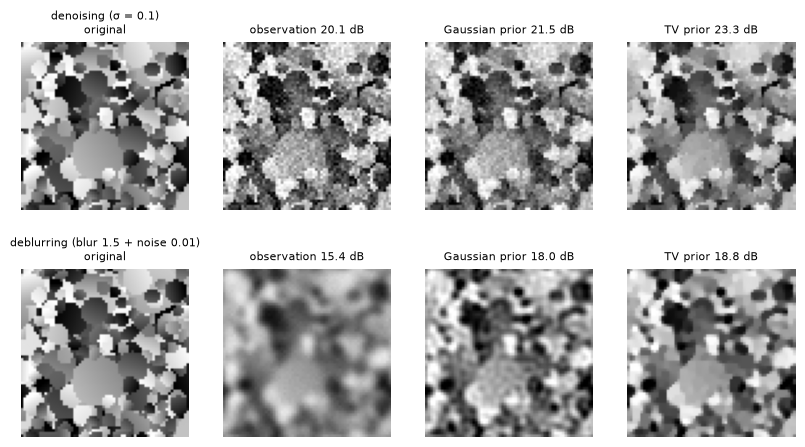
Two regularities:
-
The prior’s strength has a best value. For denoising, the PSNR of the Gaussian prior first rises, then falls with :
- : 20.09;
- : 21.50;
- : 13.17.
Too weak, and the noise stays; too strong, and the image is smeared flat. This is the same trade-off as the bandwidth of kernel density estimation in Lecture 1.
-
The prior’s shape matters more. The Gaussian prior punishes large gradients too harshly and blurs the edges too (third column of the figure). The TV prior keeps the edges and denoises about 1.7 dB better. For deblurring TV is only about 0.8 dB better: the blur has already destroyed most of the edge information, and “sparse gradients” alone cannot bring it back.
The rest of this lecture searches for priors with “a more correct shape”: from hand-designed TV, to GMMs learned from data, to the network architecture itself.
1.5 Super-resolution: the “null space” of the observation
Super-resolution shows one-to-many most plainly. Part 3 of code 01 averages every 2×2 block of the 64×64 original, giving a 32×32 low-resolution image. It then builds four completely different high-resolution images:
- the original;
- the original plus 0.2 × a ±1 checkerboard;
- the original plus 0.3 × vertical stripes;
- each low-resolution pixel copied into a 2×2 block.
All four downsample to exactly the same low-resolution image (maximum difference ), yet their PSNR against the original ranges from ∞ down to 10.46 dB.
The reason: downsampling only records “the mean of every 2×2 block”. The other 3 degrees of freedom inside a block (patterns that “sum to zero within the block”, such as checkerboards and horizontal or vertical stripes) are completely invisible to the observation. They form the null space of the downsampling operator. The data term treats components in the null space all alike; only the prior can say “a checkerboard does not look like a natural image”.
The prior’s job is to decide for us in the directions where “the observation cannot tell”. The more ill-posed the restoration problem, the more the prior matters.
2. Statistics of natural images
2.1 Power spectrum:
The power spectrum of natural images (squared magnitudes of the Fourier coefficients, averaged over frequency radius) falls off roughly as (Field 1987; Ruderman & Bialek 1994). On a log-log plot it is a line with slope about −2. Low frequencies (large-scale brightness) carry much energy, high frequencies (details) little, and the decay is a power law — there is no “characteristic scale”.
Part 1 of code 02: the power-spectrum slope of the dead leaves images is −2.02, in line with natural images.
2.2 A counterexample: Gaussian images with the same power spectrum
Now the key experiment. We build “Gaussian twins”: multiply the Fourier transform of white noise by the square root of the mean power spectrum of the dead leaves images and transform back. The result has exactly the same power spectrum as the dead leaves images (slope −2.04), but completely random phases.
Why does this experiment matter? A stationary Gaussian distribution is fully determined by its mean and covariance, and the covariance of a stationary image (after a Fourier transform) is its power spectrum. So these images are what “the best single Gaussian prior” can generate.
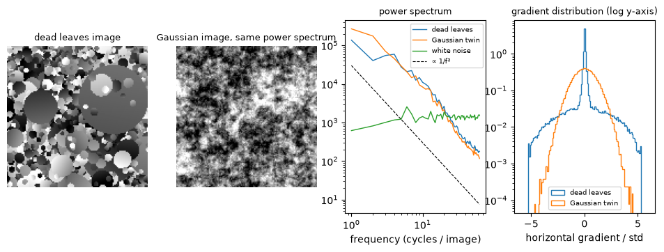
The two kinds of images have identical second-order statistics, yet look worlds apart. The dead leaves images have flat regions and sharp edges; the Gaussian twins are clouds of fog.
2.3 Heavy-tailed gradients and contrast variation
The best way to quantify the difference is the distribution of gradients (differences of neighbouring pixels) (code 02):
| images | power-spectrum slope | gradient kurtosis | gradient | gradient |
|---|---|---|---|---|
| dead leaves | −2.02 | 11.6 | 63.9% | 3.99% |
| Gaussian, same power spectrum | −2.04 | 3.1 | 8.1% | 0.30% |
| white noise | +0.06 | 3.0 | 8.0% | 0.28% |
(A Gaussian has kurtosis 3, , .)
The gradient distribution of the dead leaves images is heavy-tailed: over 60% of gradients are almost zero (leaf interiors are flat), and a few are very large (leaf edges). Natural images behave the same way (Mallat 1989; Olshausen & Field 1996’s sparse coding starts exactly here). This is why the TV prior beat the Gaussian prior in §1.4: its assumption “gradients are Laplace” is closer to the truth.
The second regularity is contrast variation (part 4 of code 02):
- Dead leaves: the standard deviations of 8×8 patches vary a lot (coefficient of variation 0.50). Some patches fall entirely inside one leaf and are almost flat (5% have std below 0.02); others straddle an edge with high contrast.
- Gaussian twins: every patch has about the same contrast (coefficient of variation 0.21, not a single flat patch).
“Contrast varies from patch to patch” means the coefficients in all directions “grow and shrink together”. That is a higher-order dependency no single Gaussian can represent; we will see how a Gaussian scale mixture (GSM) and a Gaussian mixture (GMM) represent it.
A Gaussian prior can only represent second-order statistics (the power spectrum), while the most important structures of natural images — edges, flat regions, contrast variation — all live in higher-order statistics.
2.4 Scale invariance — and where our toy fails
Natural images are approximately scale invariant over a wide range of scales: shrink a photo and its statistical regularities barely change (Ruderman 1994). In theory, with leaf sizes covering an infinitely wide range, the dead leaves model is exactly scale invariant: after shrinking, large leaves become medium ones and medium ones small, and the statistics are unchanged (Lee, Mumford & Huang 2001).
But part 3 of code 02 shows honestly that our dead leaves images are not scale invariant. After shrinking 2× and 4×:
- the gradient kurtosis falls from 11.6 to 6.6 and 4.1;
- the power-spectrum slope flattens from −2.02 to −1.42.
The reason is the minimum leaf size (radius 2 pixels). After shrinking 4×, many small leaves become smaller than a pixel and are averaged into “texture”, so the gradients are no longer sparse.
The toy captures “occlusion + heavy tails” but not full scale invariance. Fortunately, all experiments of this lecture are done at a single scale, so this flaw does not affect the later conclusions.
3. Patch priors: from PCA to Gaussian mixtures
3.1 Why learn on small patches
Learning a directly for whole images (hundreds of thousands of dimensions) was unrealistic in 2011: learning, inference and computing likelihoods were all extremely hard. Markov random fields (MRFs, e.g. Roth & Black’s Fields of Experts) tried, but their normalizing constants cannot be computed, so even the likelihood can only be approximated.
Small patches (say 8×8 = 64 dimensions) are much easier. Millions of patches can be taken from images as training data, and almost any model can compute exact likelihoods and MAP estimates. The EPLL paper opens with three questions:
- Do priors with higher likelihood on patches also give better patch restoration (denoising)?
- Applied to whole images, do they also restore better?
- Can better patch priors be learned?
The paper’s procedure: take random 8×8 patches from the training images of the Berkeley dataset and remove each patch’s mean (DC). The mean brightness is mostly determined by “what color this leaf / object is”, which has nothing to do with “what structure is in the patch”. The DC is added back during restoration.
(One implementation detail: after removing the DC, the 64 pixels always sum to 0 and the data occupy only 63 dimensions. A full-covariance Gaussian fitted in 64 dimensions has zero variance in the 64th direction, and its density is undefined. The code of these notes replaces every patch by “its 63 orthonormal DCT coefficients other than the DC” — an orthonormal coordinate system that preserves lengths, distances and white noise; see image_priors.dct_basis.)
3.2 A sequence of increasingly strong patch priors
Table 1 of the EPLL paper and Figure 1 of the 2012 paper compare a sequence of models, roughly from weak to strong:
| model | assumption | what it can represent |
|---|---|---|
| independent pixels | every pixel independent | no structure at all |
| multivariate Gaussian (MVG) / PCA + Gaussian | one full-covariance Gaussian | second-order statistics (the power spectrum) |
| PCA / ICA + non-Gaussian marginals | the outputs of some set of linear filters are independent, each heavy-tailed | sparsity (large responses at edges, zero elsewhere) |
| Gaussian scale mixture (GSM) | , Gaussian, a random contrast | contrast variation |
| Gaussian mixture (GMM) | , full covariances, nothing constrained | contrast + different “kinds” of structure |
The paper reports (EPLL Table 1, 8×8 patches, noise ):
| model | test log-likelihood | patch-denoising PSNR (MAP, dB) |
|---|---|---|
| independent pixels | 78.26 | 24.43 |
| MVG | 91.89 | 26.81 |
| PCA | 114.24 | 28.38 |
| ICA | 115.86 | 28.49 |
| GMM (200 components) | 164.52 | 30.29 |
The higher the likelihood, the better the denoising — the answer to the first question.
The 2012 paper goes further. The 200-component GMM beats (or ties) every model of the time in likelihood, including GSMs, MoGSMs, overcomplete sparse coding and the Karklin–Lewicki model. Moreover, many of these models can themselves be written as GMMs “with exponentially many or infinitely many components and constrained covariances”. That an unconstrained GMM with only 200 components beats them all is what the paper finds “surprising”.
GMMs are trained with the EM algorithm (Lecture 3 presents EM as “coordinate ascent on the ELBO”):
- the E-step computes each patch’s posterior over components, ;
- the M-step re-estimates weighted by .
The paper reports 30 hours of training on 2 million patches (unoptimized MATLAB). We train on 40,000 patches, and even K = 128 takes only tens of seconds.
3.3 Experiment: likelihood and denoising
Code 03 reproduces this curve on 8×8 dead leaves patches (63 DCT coefficients):
| patch prior | test log-likelihood (nat / patch) | MAP denoising PSNR (dB, ) |
|---|---|---|
| independent Gaussian coefficients | 27.63 | 21.82 |
| independent Laplace coefficients (sparse) | 29.67 | 21.37 |
| one full-covariance Gaussian (K = 1) | 28.03 | 21.83 |
| GMM, K = 2 | 35.58 | 22.05 |
| GMM, K = 8 | 46.02 | 22.32 |
| GMM, K = 32 | 56.13 | 22.53 |
| GMM, K = 128 | 59.47 | 22.59 |
| (the noisy patches themselves) | — | 20.07 |
(The results for K = 4, 16 and 64 lie in between; see the code output. The correlation between likelihood and PSNR over the 10 models is 0.917.)
- From K = 2 on, the GMM leaves every “single distribution” behind. The larger K, the higher the likelihood and the better the denoising, but the gains shrink — in agreement with the paper.
- One full-covariance Gaussian is only slightly better than “independent coefficients”. For stationary images the DCT already almost decorrelates the coefficients (DCT ≈ PCA), so a full covariance has little second-order correlation left to capture.
- One difference from the paper: the independent Laplace prior has a higher likelihood than the Gaussian (heavy tails), yet its MAP denoising is the worst.
- Its MAP is per-coefficient soft thresholding, , which sets many small coefficients straight to zero and over-smooths.
- In Table 1 of the paper, MAP with “PCA + non-Gaussian marginals” beats the Gaussian; on our dead leaves patches it does not.
- “Higher likelihood, better restoration” is an overall trend, not a theorem.
3.4 What the GMM learns (Zoran & Weiss 2012)
The GMM as a generative process. Sampling from a GMM takes two steps:
- pick a component according to (the nonlinear step);
- sample from (the linear step): with , where are the eigenvectors and eigenvalues of .
So every component is a “dictionary”: the eigenvectors are its “entries” (basis images), and the eigenvalues decide how strongly each entry is used. To understand what a component captures, look at the eigenvectors and eigenvalues of its covariance.
This is also one of the angles from which the EPLL paper discusses GMMs. The eigenvectors of all components together form a huge dictionary, but each patch may only use the entries of a single component — an extremely constrained kind of “sparse representation”.
The paper’s analysis has three layers:
- Contrast. In a two-component GMM, the two components have almost the same eigenvectors and the same shape of eigenvalue spectrum, differing only by a factor — exactly a GSM (). A GMM with 8–10 components already matches a GSM with 16. So the first few GMM components learn “contrast variation”. “Factorized” models such as ICA cannot represent this, because contrast scales all coefficients together.
- Texture. With more components, sorted by weight, the first few dozen are mostly “Fourier-like” components: similar eigenvectors, different eigenvalue spectra — textures of different scales and orientations.
- Boundaries. A rarer group of components has principal eigenvectors whose structure is concentrated on one side of the patch: Fourier-like structure on one side, almost zero on the other — patches whose two sides, across an edge, carry different textures.
The mini dead leaves model explains all of this. The paper proposes a patch-level generative process:
- Flip a coin to decide whether the patch is a “flat patch” or an “edge patch”.
- A flat patch = a random mean + contrast × a stationary texture (a GSM).
- An edge patch = a line with random angle and position splits the patch into two halves, each half taken from an independent flat patch.
Given the latents (flat or edge, contrast, position of the line), the patch is a Gaussian with a completely known covariance — the mini dead leaves model is itself a GMM.
Moreover, in an edge patch the pixels belonging to the two objects are independent, so the corresponding covariance entries are zero. After reordering the pixels by object, the covariance is block diagonal, and its eigenvectors are “the Fourier basis of a stationary texture on one side, zero on the other” — exactly what the boundary components learned on natural images look like.
On mini-dead-leaves data, the GMM’s likelihood also beats PCA, ICA and GSM by a wide margin. PCA and ICA look for linear transforms, but occlusion is nonlinear; a GSM captures contrast but not occlusion.
The paper’s conclusion: GMMs are strong because they represent both contrast and occlusion. (The paper also admits that the mini dead leaves model itself is only about 0.1 bit / pixel better than a GSM, equivalent to a 32-component GMM and much worse than one with 200 components. It explains the main structure the GMM learns, but it is not a better image model.)
3.5 Experiment: testing these claims on dead leaves patches
Part 3 of code 03 runs the same analysis on our dead leaves patches. The results partly agree:
-
K = 2: the total variances of the two components differ by a factor of 23.8 (one low-contrast, one high-contrast), but their “shapes” do not differ by just a factor:
- ;
- the subspaces spanned by the top 10 eigenvectors overlap only 0.45 (random subspaces: about 0.16).
The low-contrast component is mostly lighting gradients inside leaves and sensor noise; the high-contrast one is edges. In our toy, “flat” and “edge” patches are too different to be “the same structure at different contrasts” as in natural images.
-
K = 64: grouped by contrast and “one-sidedness” (the fraction of the top 3 eigenvectors’ energy concentrated in one half of the patch):
| component group | count | total weight | total variance (median) | one-sidedness (median) |
|---|---|---|---|---|
| flat patches (total variance < 0.2) | 1 | 0.095 | 0.051 | 0.59 |
| boundary patches (one-sidedness ≥ 0.75) | 4 | 0.155 | 1.661 | 0.86 |
| structure across the whole patch | 18 | 0.721 | 3.868 | 0.54 |
| almost unused (weight < 0.3%) | 41 | 0.029 | 1.689 | 0.60 |
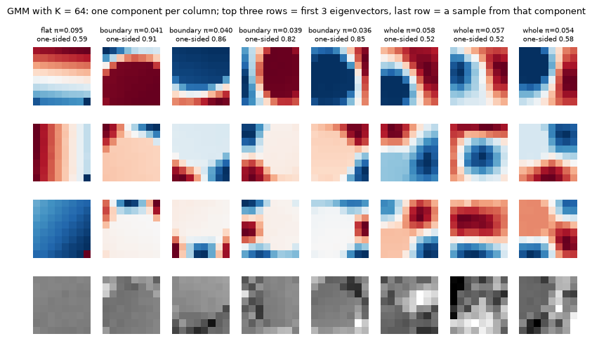
The figure shows it most clearly:
- the principal eigenvector of a boundary component is an “occlusion mask”: an arc-shaped region becomes brighter or darker as a whole, while the other side stays put. This is exactly the prediction of the mini dead leaves model: two leaves occupy the two sides of the patch, and the main variation is “the brightness difference between the two leaves”;
- the eigenvectors of the flat component are smooth brightness gradients (the lighting inside a leaf).
Unlike in the paper, boundary components are not particularly rare here (the correlation between one-sidedness and weight is −0.08). Also, 41 of the 64 components are almost unused. For 40,000 training patches, 64 full-covariance components are already more than the data really need (a common phenomenon with EM).
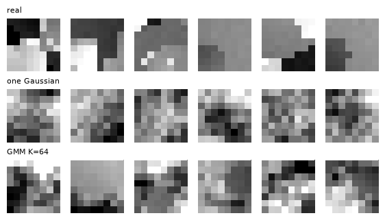
Sampling (part 4 of code 03). The within-patch kurtosis of horizontal gradients is:
- real patches: 10.0;
- samples of a single Gaussian: 3.0 (it only knows the power spectrum);
- samples of the GMM: 5.3.
GMM samples have flat regions and edges: the GMM has learned far more structure than second-order statistics, but is still some way from the real distribution.
4. From patches to whole images: EPLL
4.1 The problem: how to apply a patch prior to a whole image
Given a good patch prior, how do we restore a whole image? Figure 2 of the EPLL paper uses a minimal example to show the problems of several naive approaches:
- Non-overlapping patches: cut the image into non-overlapping patches, MAP-denoise each, and put them back. Clear seams appear at the patch borders: in the stitched image, patches that straddle a seam “do not exist” under the prior.
- Center pixel only: denoise every overlapping patch and use only its center pixel.
- Patch averaging: denoise all overlapping patches independently and give every pixel the average over all patches covering it. This is what most patch methods of the time did (KSVD, BM3D, LLSC, …). It is better, but still flawed: averaging independently denoised patches creates new patches, and these new patches are not likely under the prior.
4.2 EPLL: make every patch likely
The idea of EPLL is direct. The prior describes “what a patch at a random location should look like”, so require every patch of the restored image (all overlapping patches) to be likely under the prior, while staying close to the observation. Define the Expected Patch Log Likelihood:
where extracts the -th patch (all overlapping patches). The restoration cost is
The paper stresses that is not the log-probability of the whole image. It “double counts” the probability of the overlaps; it is the expected log-likelihood of “a patch at a randomly chosen location” (up to a factor ). This is a very clever engineering compromise: instead of learning a whole-image model (which cannot be learned), learn only a patch model, then “stitch” patches together with a sensible objective.
4.3 Half-quadratic splitting: alternate two simple things
Optimizing directly is hard ( is the log of a GMM, non-convex). The paper uses half-quadratic splitting (Geman & Yang 1995): introduce an auxiliary variable for every patch and rewrite the cost as
As this forces , recovering the original problem. For a fixed , alternate between two sub-problems:
- -step (fix ): a quadratic function; setting the derivative to zero gives the closed form For denoising, and is diagonal (how many patches cover each pixel). So is a per-pixel weighted average of “the observation ” and “the average of all put back in place”. For inpainting, (the mask): the term vanishes at missing pixels, which are determined entirely by the patches.
- -step (fix ): for every patch independently, solve . This is exactly “treat as a noisy observation (variance ) and MAP-denoise it with the prior ”.
Then increase and alternate again. The paper uses and ( is the number of pixels in a patch). Two points are worth noting:
- As long as each sub-problem “improves”, the original objective is being optimized — exact solutions are not required. Figure 3 of the paper shows that the cost still decreases even when the -step uses the posterior mean (BLS) instead of the MAP.
- In the first round () with initialization , EPLL is almost exactly patch averaging. After that it repeatedly “re-extracts patches from the current restoration and denoises them again”, while gradually tightening the requirement “patch = denoised patch”.
The -step for a GMM. Under a GMM prior the MAP of a patch has no closed form. The paper uses an approximation:
- compute the posterior of the noisy patch over the components (component covariance plus noise variance);
- pick the component with the largest posterior;
- Wiener-filter with that component:
This is one step of “hard EM for finding the mode of a GMM”.
4.4 What the paper reports
-
EPLL improves every prior (Figure 4 and Table 1 of the paper). Whole-image denoising PSNR () with the same prior, patch averaging vs EPLL:
- MVG 27.14 vs 27.71;
- ICA 29.02 vs 29.53;
- GMM 29.59 vs 29.85.
Priors with higher likelihood also give better whole-image restoration — the answer to the second question.
-
The best generic prior of its time. On 68 Berkeley test images (Table 2 of the paper), GMM + EPLL is the best generic prior method (: 28.71 dB, vs KSVDG 28.28 and FoE 27.77). It is also on par with methods that learn from the noisy image itself (BM3D 28.57, LLSC 28.70).
-
Deblurring (known blur kernel): about 1.3 dB above Krishnan & Fergus’s hyper-Laplacian prior (27.17 vs 25.84, 27.70 vs 26.38). Deblurring cannot average away noise using “similar patches elsewhere in the image” as denoising can, so a generic prior is especially useful here.
-
Cost: about 300 seconds per image (unoptimized MATLAB), 4–5 times patch averaging.
4.5 Experiment: on dead leaves images
Code 04, on 4 unseen 64×64 dead leaves images ():
| method | mean PSNR | mean of patches in the result |
|---|---|---|
| noisy image | 20.00 | 14.6 |
| single Gaussian prior, patch averaging | 21.96 | 31.8 |
| single Gaussian prior, EPLL | 21.51 | 26.7 |
| GMM prior, non-overlapping patches | 22.91 | 61.7 |
| GMM prior, patch averaging | 23.76 | 65.5 |
| GMM prior, EPLL (paper setting ) | 23.34 | 69.4 |
| GMM prior, EPLL ( reduced to 1/4) | 24.02 | 89.4 |
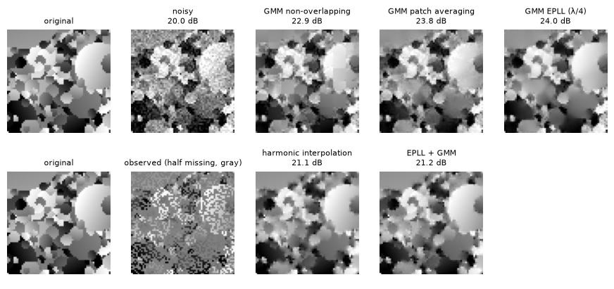
- The better the prior, the better the restoration: every use of the GMM beats every use of the single Gaussian (by about 1–2 dB).
- How it is used also matters: non-overlapping patches are about 0.9 dB below patch averaging (seams).
- EPLL really does optimize “every patch is likely”: its restorations have the highest mean of patches (69.4 and 89.4, vs 65.5 for patch averaging). As increases, PSNR and the patches’ rise together (, image 1: 23.08 → 23.79 → … → 24.04 dB).
- But: with the paper’s default hyperparameters, EPLL on our dead leaves images is about 0.4 dB below patch averaging. Only with the data-term weight reduced to 1/4 is it about 0.3 dB above.
- The paper’s schedule was hand-tuned on 5 natural images and need not suit other data; such half-quadratic splitting methods are quite sensitive to their hyperparameters.
- This is the clearest disagreement between the toy results of these notes and the paper’s conclusions, and we keep it as it is.
Inpainting (part 2 of code 04, half of the pixels removed at random). Inpainting is just denoising with “different noise at every pixel”: missing pixels have infinite noise. Replace by in EPLL’s -step and the framework needs no other change.
We start from harmonic interpolation (repeatedly set missing pixels to the mean of their four neighbours, corresponding to a “smooth everywhere” prior). EPLL + GMM is a little better on every image, but only by 0.02–0.16 dB. With half of the pixels missing at random, most neighbours of a missing pixel are observed, and simple smooth interpolation is already strong.
4.6 EPLL’s legacy
EPLL’s “alternate two things” — one step pulls the result toward the observation (-step), the other denoises with the prior (-step) — later became a very general idea:
- Plug-and-Play priors (Venkatakrishnan et al. 2013): the -step only needs a “denoiser”, so any denoiser (BM3D, later neural networks) can be plugged in as the prior, for any inverse problem.
- Solving inverse problems with diffusion models (much work after Lectures 12–14): a diffusion model is itself a prior that “can denoise at every noise level”, and the structure “alternately move toward the observation, then denoise” descends directly from EPLL.
But EPLL, like every method of this lecture, gives only one answer (the MAP). As Lecture 1 said, restoration is a one-to-many problem; the generative models later in the course sample from the posterior and give several plausible answers.
5. Non-parametric methods (optional)
5.1 Efros–Leung texture synthesis (1999)
Lecture 1 §1.2 introduced this algorithm; now we look at its details and experiments. The paper starts from Shannon’s use of -grams to generate “English-like” text: knowing the previous letters, sample the next one from corpus statistics. Efros and Leung wanted to extend this to 2-D textures, which means answering three questions:
-
what is the unit of synthesis (a pixel);
-
what is the context (the known pixels in a square window around it);
-
how is the conditional distribution built.
-
Model assumption: a texture is a Markov random field — given its neighbours in a square window, a pixel’s brightness is independent of the rest of the image. The window size is the only user parameter. It should be about as large as “the largest regular structure” in the texture: a small window learns only local randomness, a large one learns the overall regular arrangement (Figure 2 of the paper).
-
The conditional distribution is not modeled explicitly. For a pixel to synthesize, find all locations in the example whose neighbourhoods are similar enough to its (known) neighbourhood:
- “similar enough” means a distance within times the smallest distance (the paper uses );
- distances are Gaussian-weighted (, nearby pixels matter more).
The center pixels of these locations form a histogram, which approximates the conditional distribution; sample from it.
-
Order: start from a 3×3 seed and “grow” outward layer by layer; pixels with more known neighbours are synthesized first (a “Shannon-style” heuristic). The paper says that repeatedly correcting with Gibbs sampling brings almost no improvement.
-
Failure modes (Figure 5 of the paper): sometimes it “slips” into the wrong region of the example and starts “growing garbage”; sometimes it gets stuck at one place in the example and starts copying it verbatim.
In today’s language: this is an autoregressive model that generates pixel by pixel in a fixed order, sampling at every step from a non-parametric conditional distribution.
Experiment (part 1 of code 05). We synthesize 48×48 outputs from two 32×32 examples, bricks and dead leaves, and compare three methods:
- pick one at random (the paper);
- always the most similar (the mode);
- average the similar-enough ones (regression).
is swept from 0.1 to 1:
| example | method | sharpness (gradient / example) | neighbour pairs copied as blocks | |
|---|---|---|---|---|
| bricks | 0.1 | random / most similar / average | 1.03 / 1.02 / 1.01 | 87% / 90% / — |
| bricks | 1.0 | random / most similar / average | 1.06 / 1.02 / 0.70 | 56% / 90% / — |
| dead leaves | 0.1 | random / most similar / average | 0.91 / 0.89 / 0.91 | 56% / 57% / — |
| dead leaves | 1.0 | random / most similar / average | 1.12 / 0.89 / 0.46 | 43% / 57% / — |
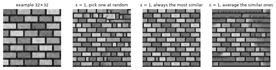
- At the only “similar enough” candidate is almost always the single most similar one, and the three methods are nearly identical.
- As grows there are more candidates: the non-parametrically estimated conditional distribution widens and becomes “one-to-many”.
- Averaging gets blurrier and blurrier (the vertical mortar lines of the bricks are smeared away), for the same reason as the ghosts of Lecture 1.
- Picking one at random stays sharp, and the fraction copied in blocks falls (it composes new arrangements). But less similar windows sneak into the candidates, and the generated windows move further from the example (errors begin).
- Always picking the most similar is unaffected by and is always the most “copied” result.
- A small aside: with “distance from a window to the nearest example window” as the ruler, averaging () is the most “similar” — per-pixel distance favours the mean once again (Lecture 1 §2.5).
5.2 PatchMatch (2009)
At the heart of many image-editing operations lies: for every small patch of image A, find the most similar patch in image B (the nearest-neighbour field, NNF). Brute force compares pairs, which makes interaction impossible for megapixel images.
PatchMatch’s insight is that natural images are highly coherent. If a patch of A has found a good match in B, its right-hand neighbour will probably find a good match just to the right of that location. The algorithm:
- Random initialization: every patch points to a random location in B.
- Propagation: in scan order, try “the match location of the left / upper neighbour, shifted one step right / down”; odd rounds scan in reverse.
- Random search: try a few random locations around the current best, with the radius starting at the image size and halving each time, to escape local optima.
Part 2 of code 05 (48×48 images, 7×7 patches):
| case | mean distance after 5 rounds / optimum | patches that found their true nearest neighbour | computation / brute force |
|---|---|---|---|
| B = A shifted plus noise | 1.22 | 87% | 2.3% |
| B = another dead leaves image | 1.14 | 47% | 2.3% |
- After random initialization the mean distance is 5–28 times the optimum; after one round it is only 1.4–3.4 times.
- In the shifted case, as soon as one patch “happens” to find the right location, propagation passes that good location all the way along.
- About 1/40 of the computation gets close to the optimum. On large images, that is the difference between “interactive” and “wait for hours”.
- Photoshop’s “Content-Aware Fill” uses it to find suitable patches around a hole and piece them into the hole (together with a multi-scale iterative optimization).
- (Our pure-Python loops are actually slower than the vectorized brute force: less computation, but a large Python overhead. The original paper used C++ and much larger images.)
5.3 Example-based super-resolution (Freeman et al. 2002)
The same “search the examples” idea was also used for super-resolution:
- Prepare many example pairs “low-resolution patch → corresponding high-resolution detail patch”.
- For a new low-resolution image, look up at every position the example patches whose low-resolution parts are most similar.
- Pick a high-resolution detail that is compatible in the overlap with the neighbouring patches already chosen. The paper models this compatibility with a Markov network and gives a fast one-pass approximation.
Like Efros–Leung and PatchMatch, its “prior” is the example library itself — a non-parametric .
The strength of non-parametric methods: no modeling, realistic details. Their weakness: they can only “copy” existing fragments, generalize poorly, and must store and search all examples (the experiment of Lecture 1 §2.6: the data needed for copying nearest neighbours grows rapidly with the number of style dimensions). What deep generative models do is “compress” these conditional distributions into a parametric network that generalizes.
6. Deep Image Prior: the architecture is the prior
6.1 A counter-intuitive question
By 2018, convolutional networks led across the board in denoising, super-resolution and similar tasks. The usual belief was that this was because they “learned realistic priors from large numbers of images”. Ulyanov, Vedaldi and Lempitsky wanted to know: before any learning, how much does the network architecture itself contribute?
They cite the finding of Zhang et al. (2017): the same classification network can both generalize on true labels and completely memorize random labels. So generalization requires “the structure of the network to resonate with the structure of the data”, but the nature of this resonance is unclear.
6.2 The method: re-parameterization
Write the image as the output of a generator network, :
- is a fixed random input (the paper: uniform noise the size of the image, with 32 channels);
- are the network parameters, randomly initialized and never trained on any data.
To restore, optimize on this one degraded image only:
is the data term:
- denoising: ;
- super-resolution: ( is downsampling);
- inpainting: .
Compare with the MAP of §1.3. The regularizer of is replaced by ” must be an image this network can produce” — formally (can produce) or (cannot). Like TV, this prior is “hand-designed”; only what is designed is the network architecture. The default network is a U-Net-style “hourglass” with skip connections and about 2 million parameters.
6.3 Why a network that “can fit anything” can serve as a prior: impedance
A two-million-parameter network can of course fit any image, including pure noise — so why can it still act as a “prior”?
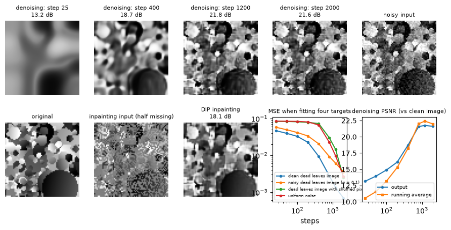
The paper’s key experiment (Figure 2) lets the network fit four targets and watches how fast the loss falls:
- a natural image;
- a natural image + noise;
- an image with shuffled pixels;
- white noise.
The natural image falls much faster; noise and the shuffled image fall very slowly. In the paper’s words, the parameterization has “low impedance to signal and high impedance to noise”: the network can eventually fit unstructured noise too, “only very reluctantly”. So as long as we stop early, we get a result where “the structure has been fitted but the noise not yet”.
Experiment (part 1 of code 06; our network is a small hourglass of about 120,000 parameters without skip connections, 64×64):
| target | 100 steps | 400 steps | 800 steps | 2000 steps |
|---|---|---|---|---|
| clean dead leaves image | 0.0327 | 0.0094 | 0.0028 | 0.0007 |
| noisy dead leaves image () | 0.0415 | 0.0205 | 0.0092 | 0.0036 |
| dead leaves image with shuffled pixels | 0.0814 | 0.0728 | 0.0297 | 0.0025 |
| uniform noise | 0.0833 | 0.0664 | 0.0224 | 0.0026 |
(Entries are the MSE to the target.)
- In the first 400 steps the shuffled image and pure noise hardly move, while the error on the clean image has already dropped by an order of magnitude.
- After 800 steps the network starts fitting them too, and at 2000 steps all errors are small.
The shuffled image has exactly the same distribution of pixel values as the original, just no spatial structure — and spatial structure is exactly what the network “prefers”. The difference lies mainly in speed, as the paper describes.
6.4 Denoising: rise, then fall — early stopping is a must
Part 2 of code 06 fits the noisy image but watches the PSNR of the output against the clean image:
| steps | 25 | 200 | 400 | 800 | 1200 | 2000 |
|---|---|---|---|---|---|---|
| PSNR of the output | 13.17 | 16.11 | 18.69 | 21.57 | 21.76 | 21.61 |
| PSNR of the running average | 10.56 | 15.28 | 18.20 | 22.01 | 22.42 | 21.99 |
-
The PSNR rises, then falls. The network first fits the structure of the image (coarse to fine, top row of the figure), then slowly fits the noise too. The number of iterations is itself the strength of the regularization, so early stopping is a must. This is also Deep Image Prior’s biggest weakness: in real use there is no clean image, and we do not know when to stop.
-
Output averaging. One trick from the paper is an exponential moving average of the outputs of recent iterations. In our experiment the running average lags early on (it “remembers” the early blurry images), and after 800 steps it is 0.4–0.7 dB better than the current output.
-
Compared with EPLL: on the same image, EPLL + GMM reaches 23.51 dB, while DIP at best reaches 22.42 dB. A small network — a “hand-made prior” with untuned architecture and hyperparameters — cannot match a prior learned from 40 images of the same kind.
-
What the paper reports on natural images (DIP is close to, but below, the best classical method):
method PSNR (dB) DIP (1800 steps) 29.22 DIP + running average 30.43 DIP, two runs averaged 31.00 CBM3D 31.42 non-local means 30.26
6.5 Super-resolution and inpainting
4× super-resolution (the paper reports, Set5 / Set14, dB):
| method | Set5 | Set14 |
|---|---|---|
| DIP | 29.90 | 27.00 |
| bicubic interpolation | 28.43 | 26.05 |
| SRResNet (trained on a large dataset) | 32.10 | 28.53 |
Without any external data, DIP closes most of the gap between bicubic interpolation and learned methods.
Inpainting (the paper reports):
- on standard test images with 50% of pixels missing at random, DIP clearly beats methods based on convolutional sparse coding (e.g. Barbara: 32.22 vs 28.14 dB);
- removing text from images and filling large holes also works reasonably well.
Inpainting shows the effect of “re-parameterization” especially well. The missing pixels do not appear in the loss at all; if we optimized the pixels directly, their gradients would always be zero. Through the network, all pixels share the same convolution weights, and the missing pixels get filled “along the way” by the network’s structure.
The paper also stresses that the choice of architecture matters a great deal (Figure 8): deeper networks are better, and skip connections, so useful in recognition, are “very harmful” for tasks like filling large holes. DIP has also been used for “natural pre-images” (inverting a network’s features into images to diagnose what invariances it has learned) and for fusing flash / no-flash photo pairs.
Our experiment (part 3 of code 06, 50% of pixels missing at random) did not reproduce the inpainting success:
| method | PSNR |
|---|---|
| DIP, no skip connections (2000 steps) | 18.06 |
| DIP, with skip connections (best 17.65 at 50 steps, falling to 16.35 at 2000 steps) | 16.35 |
| harmonic interpolation | 19.66 |
| EPLL + GMM | 19.79 |
- DIP fits the observed pixels extremely well (error down to ), but guesses the missing pixels poorly — worse even than the simplest harmonic interpolation.
- With skip connections it is worse still, and gets worse with training: skip connections make it easier for the network to “fit only the observed pixels”.
This agrees with the paper’s caveat that “what an architectural prior prefers depends on the architecture itself”. The paper’s inpainting experiments use larger, deeper networks chosen for the task; with another network or another kind of data, this prior may fail.
6.6 What this paper means
The significance of Deep Image Prior is not that it is the best restoration method, but the fact it reveals: the architecture of a convolutional generator network itself carries a strong image prior. Two ingredients matter:
- convolution (local and translation equivariant);
- multi-scale upsampling (generate the coarse structure first, then add detail).
This explains why the convolutional generators of GANs and VAEs so easily produce “image-like” things. It also echoes the Lecture 1 slides: “not every part of distribution modeling is learned”.
It also builds a bridge between “learning methods” (deep networks) and “non-learning methods” (hand-made priors, self-similarity). The paper points out that DIP fills unknown parts with the textures of the known parts of the image, behaving much like a traditional self-similarity prior.
7. The big picture: three priors and the deep generative models that follow
7.1 Through the five components of Lecture 1
| GMM + EPLL | Efros–Leung / PatchMatch | Deep Image Prior | |
|---|---|---|---|
| formulation | whole image = overlapping patches; every patch independently follows the same prior (a “double-counting” approximation) | Markov random field: given its neighbourhood, a pixel is independent of the rest; generated pixel by pixel in order | image = output of a convolutional network on a fixed input |
| representation | a Gaussian mixture on 63 dims (explicit density) | the example itself (non-parametric) | the network architecture (an implicit “can / cannot produce”) |
| objective | maximum likelihood on patches (EM); MAP for restoration | none (no training) | the data term during restoration |
| optimization | EM; half-quadratic splitting | none; PatchMatch is a search algorithm | gradient descent on a single image + early stopping |
| inference | (approximate) MAP; patch likelihoods are computable | sampling (Efros–Leung); nearest neighbours (PatchMatch) | one point estimate; no likelihood |
7.2 Where they reappear later
- GMMs and latent variables. A GMM’s “pick a component first, then generate linearly within it” is a discrete latent-variable model. Lecture 3’s VAE replaces the latent with a continuous , linear generation with a neural decoder, and EM with stochastic gradient descent. Lecture 3 also covers EM itself, and K-means (a GMM “whose components all have identity covariance, with the variance going to zero”).
- Efros–Leung and autoregression. PixelRNN / PixelCNN in Lectures 5–6 represent the conditional distribution with a neural network instead of “finding neighbours in the example”. So they generalize to combinations absent from the example, and can compute exact likelihoods.
- EPLL and diffusion. EPLL’s “one step toward the observation, one step of denoising with the prior” evolved into plug-and-play priors. The diffusion model of Lecture 12 is itself a prior that “can denoise at every noise level”, and its training objective is precisely “predict the noise” — the denoiser is the prior.
- Deep Image Prior and network architecture. The GANs of Lecture 9 and the diffusion U-Nets of Lectures 12–13 all rely on the inductive biases of convolutional architectures; “what is learned and what is designed” runs through the whole course.
7.3 The most important difference: one answer vs a distribution
Every restoration method in this lecture (MAP, patch averaging, EPLL, DIP) gives only one answer. Efros–Leung is the only method that truly “samples” — and the only one the slides call a “generative model”. The deep generative models later in the course combine the two: a learned prior that generalizes, plus the ability to sample several plausible answers from the posterior .
8. Summary
- Image restoration = the inverse problem .
- Denoising, deblurring, inpainting and super-resolution differ only in .
- All are ill-posed: direct inversion amplifies noise, and super-resolution has a null space the observation cannot see at all. A prior must fill in what the data cannot tell.
- MAP = data term + . The prior’s strength must be balanced, but its shape matters more: a heavy-tailed (TV) prior beats a Gaussian prior.
- Statistics of natural images: a power spectrum, heavy-tailed gradients, contrast that varies from patch to patch, and edges created by occlusion.
- Gaussian images with the same power spectrum look nothing like natural images: a single Gaussian prior can only represent second-order statistics.
- The dead leaves model (occlusion + power-law sizes) reproduces most of these properties; our toy version is not fully scale invariant.
- Patch priors.
- Patch priors with higher likelihood usually restore better (the first finding of the EPLL paper; our Laplace prior is an exception).
- An unconstrained Gaussian mixture beats PCA, ICA, GSMs and similar models.
- It learns contrast and occlusion (Zoran & Weiss 2012): the mini dead leaves model is itself a GMM, and the eigenvectors of boundary components have “structure on one side, zero on the other”.
- EPLL.
- Require every overlapping patch of the restored image to be likely under the prior.
- Half-quadratic splitting alternates an “-step (move toward the observation, closed form)” and a “-step (MAP-denoise every patch)”, with increasing.
- In the paper it beats patch averaging across the board. On our toy it does make the patches more “likely”, but its PSNR advantage depends on the hyperparameters.
- Non-parametric methods.
- Efros–Leung represents conditional distributions non-parametrically by neighbours in the example and samples from them (a non-parametric autoregressive model). Averaging blurs; sampling stays sharp.
- PatchMatch finds approximate nearest neighbours with about 1/40 of the computation, using propagation and random search.
- Deep Image Prior.
- An untrained convolutional network has “low impedance” to natural images and “high impedance” to noise: the architecture itself is a prior.
- Early stopping is a must, and the choice of architecture matters a great deal.
- On our toy its denoising loses to EPLL, and its inpainting even loses to harmonic interpolation.
9. Common pitfalls
- “The stronger (or weaker) the prior, the better.” There is a best strength, and the shape of the prior (Gaussian vs heavy-tailed) often matters more than its strength (§1.4).
- “Second-order statistics (power spectrum / covariance) describe natural images.” Gaussian images with the same power spectrum look nothing like natural images (§2.2).
- “DC-removed patches can be fitted with a full-covariance Gaussian directly in 64 dims.” The pixels always sum to 0, the data occupy only 63 dims, and the covariance is singular (§3.1).
- “A prior with higher likelihood always restores better.” This is an overall trend, not a theorem; the properties of the MAP estimate (e.g. the soft thresholding of a Laplace prior) matter too (§3.3).
- “EPLL optimizes the log-probability of the whole image.” It is the sum of the log-probabilities of all overlapping patches, which double counts the overlaps; it is not a normalized whole-image probability (§4.2).
- “Patch averaging is a simplified EPLL with about the same results.” The new patches created by averaging need not be likely under the prior, while EPLL repeatedly re-extracts patches from the current restoration (§4.1–§4.2). But EPLL’s advantage depends on the hyperparameters (§4.5).
- “For Efros–Leung, just take the most similar one.” Always taking the most similar one tends to copy verbatim and fall into loops; averaging blurs; only random sampling stays both sharp and diverse (§5.1).
- “Deep Image Prior uses a pretrained network.” The network is fully randomly initialized and never trained on any data; the prior comes from the architecture (§6.2).
- “The longer Deep Image Prior trains, the better.” Training too long fits the noise too; early stopping is a must (§6.4).
- “All methods of this lecture are generative models.” Except Efros–Leung, they all give one MAP or point estimate and do not sample from a distribution (§7.3).
10. Exercises
Exercise 1 (the Wiener filter) Denoising in 1-D: , , prior . Show that the MAP (which is also the posterior mean) is . If is stationary (diagonalized by the Fourier basis, with eigenvalues = power spectrum ), what does this filter do at each frequency? Use this to explain why “a Gaussian prior suppresses high frequencies (including edges) when denoising”.
Answer
The posterior is . Setting the derivative in to zero gives , i.e. . The mode of a Gaussian posterior equals its mean.
In the Fourier basis, every frequency is independently multiplied by :
- low frequencies with large power are kept almost unchanged;
- high frequencies with small power are pushed close to zero.
The power of natural images falls off as , so high frequencies are strongly attenuated — and edges need exactly those high frequencies, so they are blurred. A Gaussian prior does not know that “high-frequency energy is concentrated at a few locations (edges)”.
Exercise 2 (the MAP of a Laplace prior is soft thresholding) In 1-D: , , prior . Show that the MAP estimate is . Why does this “over-smooth”? What does the posterior mean look like (qualitatively)?
Answer
Minimize .
- For the derivative is , so , which requires .
- is symmetric.
- Otherwise the subgradient at contains 0, and the solution is 0.
So all coefficients with are set to zero, and many “small but real” details are deleted.
The posterior mean is never exactly zero; it shrinks smoothly (small shrink more, large ones less) and usually has lower MSE. This is one reason why the Laplace prior in code 03 has “a high likelihood but poor MAP denoising” (Table 1 of the EPLL paper reports both BLS and MAP).
Exercise 3 (the posterior of GMM components under noisy observations)
Let a patch come from a GMM, and with . Show that , and hence . This is the meaning of extra_var in GMM.denoise_map.
Answer
Given , , and is independent of . The sum of independent Gaussians is Gaussian, with means and covariances adding: . Bayes’ rule then gives the posterior.
Intuitively: the noisier the observation, the more the noise must be taken into account when deciding “which class this patch belongs to”. Otherwise the noise is mistaken for high-contrast structure, and the patch is misassigned to a high-contrast component.
Exercise 4 (EPLL’s -step) Differentiate to derive the closed form of §4.3. For denoising (), show that it reduces to the per-pixel , where is the number of patches covering pixel .
Answer
, i.e. .
- is a diagonal matrix with 1 on the pixels covered by patch , so .
- With the left-hand side is the diagonal matrix ; dividing pixel by pixel gives the result.
- at pixel is the sum of the values at that position of all patches covering it — exactly the
accreturned byfold_patches.
Exercise 5 (why EPLL is not a whole-image likelihood) Let an image have just 1 row of 3 pixels, and let the “patches” be windows of length 2. Write . Under what condition does it equal plus a constant?
Answer
Suppose form a Markov chain ( and independent given ). Then , so .
The remaining term depends on ; it is not a constant. So EPLL “counts” the middle one extra time. Even under the ideal Markov condition, EPLL is only an approximation of the whole-image likelihood. Its value lies in the intuitive, practical requirement “every patch is likely”.
Exercise 6 (Efros–Leung and autoregression) Write Efros–Leung in the autoregressive form of Lecture 1: what is the generation order? How is the conditional distribution represented? Why does it “need no training”? Compared with representing the same conditional with a PixelCNN, what are the pros and cons of each?
Answer
- Order: layer by layer outward from the seed, pixels with more known neighbours first.
- Conditional distribution: the histogram of the center pixels of all example windows similar enough to the known neighbours (a non-parametric empirical distribution).
- No training, because the “model” is the example itself: the conditional distribution is built on the fly at each query.
- Pros: details come entirely from a real example and are realistic; no training is needed.
- Cons:
- it can only copy local combinations that occur in the example, so it cannot generalize;
- every generated pixel requires searching the whole example (slow);
- there is no explicit likelihood;
- the window size and must be tuned by hand.
PixelCNN represents the conditional distribution with one network with shared parameters. It generalizes and computes likelihoods, at the price of training and possibly less realistic detail.
Exercise 7 (the parameter count of Deep Image Prior) Our hourglass network has about 120,000 parameters, and an image has 64×64 = 4096 pixels. The network has almost 30 times as many parameters as pixels. By the intuition “many parameters can fit anything”, why can it still act as a prior? Which number in part 1 of code 06 makes the point best?
Answer
Many parameters mean “can eventually fit”, but the prior effect comes from the optimization path. Gradient descent from a random initialization first fits the image components the network “produces easily” (low frequencies, spatially structured parts), and only later those it does not (noise, shuffled images). So the prior is determined jointly by “architecture + optimization + early stopping”.
The number that makes the point best is the error at 400 steps: clean image 0.0094, shuffled image 0.0728. The pixel-value distributions are identical and only the spatial structure differs, yet the fitting speed differs by almost 8×.
Exercise 8 (hands-on)
(a) In 03_patch_gmm.py, change the patch size from 8×8 to 6×6 (you need to change dct_basis and the patch extraction). How does the likelihood vs number-of-components curve of the GMM change?
(b) In 04_epll.py, replace the β schedule by the denser (1, 2, 3, 4, 6, 8, 12, 16, 24, 32, 48, 64). Can EPLL (with the paper’s λ) catch up with patch averaging?
(c) In 06_deep_image_prior.py, change the learning rate from 0.01 to 0.001. How do the best number of steps and the best PSNR for denoising change?
Answer (sketch)
(a) Smaller patches have lower dimension: the per-dimension likelihood is usually higher and fewer components are needed. But the patches can represent less structure (coarser edge orientations and occlusion shapes). For restoration, smaller patches carry less context, and results are usually a little worse.
(b) Tried while writing these notes: the denser β schedule brings EPLL with the paper’s setting roughly level with patch averaging (about 23.77 dB). It converges more fully, but still does not beat reducing λ. Trust your own run for the exact numbers.
(c) With a smaller learning rate the fit is slower, and the process “fit the structure first, the noise later” is stretched out, so the best number of steps moves later. The best PSNR may be similar, but the early-stopping “window” is wider and easier to hit.
11. Further reading
Required and optional papers
- D. Zoran & Y. Weiss, From Learning Models of Natural Image Patches to Whole Image Restoration, ICCV 2011.
- D. Zoran & Y. Weiss, Natural Images, Gaussian Mixtures and Dead Leaves, NeurIPS 2012.
- D. Ulyanov, A. Vedaldi, V. Lempitsky, Deep Image Prior, CVPR 2018.
- A. A. Efros & T. K. Leung, Texture Synthesis by Non-parametric Sampling, ICCV 1999.
- C. Barnes, E. Shechtman, A. Finkelstein, D. B. Goldman, PatchMatch, SIGGRAPH 2009.
- W. T. Freeman, T. R. Jones, E. C. Pasztor, Example-Based Super-Resolution, IEEE Computer Graphics and Applications, 2002.
Background
- D. J. Field, Relations between the statistics of natural images and the response properties of cortical cells, JOSA A 1987; D. L. Ruderman, The statistics of natural images, Network 1994: and scale invariance.
- A. B. Lee, D. Mumford, J. Huang, Occlusion Models for Natural Images: A Statistical Study of a Scale-Invariant Dead Leaves Model, IJCV 2001.
- B. A. Olshausen & D. J. Field, Emergence of simple-cell receptive field properties by learning a sparse code for natural images, Nature 1996: sparse coding.
- M. J. Wainwright & E. P. Simoncelli, Scale Mixtures of Gaussians and the Statistics of Natural Images, NeurIPS 1999: GSMs.
- L. Rudin, S. Osher, E. Fatemi, Nonlinear total variation based noise removal algorithms, Physica D 1992: TV.
- S. Roth & M. J. Black, Fields of Experts, IJCV 2009: learned MRF priors.
- K. Dabov et al., Image Denoising by Sparse 3-D Transform-Domain Collaborative Filtering (BM3D), TIP 2007: non-local patch methods.
- S. V. Venkatakrishnan, C. A. Bouman, B. Wohlberg, Plug-and-Play Priors for Model Based Reconstruction, GlobalSIP 2013: denoisers as priors.
Related notes in this course
- Prerequisite P1 §2 (conditionals of Gaussians, the KL between two Gaussians), §6 (change of variables); Prerequisite P2 §3 (convolutions, U-Nets).
- Lecture 1 §1.2–§1.3 (the historical place of Efros–Leung and PatchMatch), §2 (one-to-many and ghosts).
12. Next lecture
Lecture 3: Variational autoencoders (VAE), EM and VQ-VAE (original lecture · 09/12; original Pset 1).
The GMM of this lecture is a latent-variable model that “first picks a discrete component, then generates linearly within it”, trained with EM. Lecture 3 generalizes it all the way:
- The latent becomes a continuous , and “linear generation” becomes a neural decoder . Representational power grows enormously, but the posterior no longer has a closed form.
- So we introduce a “controllable” distribution and derive the ELBO (P1 §4.3 already verified numerically). It is parameterized by an encoder network and trained with the reparameterization trick.
- Then we revisit EM (coordinate ascent on the ELBO) and K-means (a special case of EM, and also an autoencoder). Finally comes VQ-VAE, which turns the discrete “component choice” into an image tokenizer.