Maps to: MIT 6.S978 Deep Generative Models (Fall 2024), Lecture · Thu 10/03/2024 · Generative Adversarial Network (GAN) (slides:
lec4_gan.pdf, Kaiming He). Problem Set 3 (released 10/08):
- an unconditional MLP GAN on MNIST, three ablations and a conditional GAN;
- derivations of the optimal discriminator and the global optimum;
- Kantorovich–Rubinstein duality in discrete optimal transport.
Basis: The order and content follow the slides: GAN, Wasserstein GAN, the adversary as a loss function. The derivations the slides cite (“see proof in Goodfellow et al.”) are written out in full, and all of Problem Set 3 is done: the coding problems on glyphs instead of MNIST (§4.4), the derivations as worked solutions (§3, §5.3, exercises). Experiments were designed for these notes and run on a CPU. Several outcomes differ from the textbook story and are reported as they came out:
- the original “minimax” loss covered more modes than the non-saturating one on our 2-D toy;
- WGAN with the paper’s clipping settings barely trained;
- Problem Set 3’s MLP GAN collapsed onto a few digits in every unconditional run.
Code:
code/lecture09/— 5 scripts + the shared modulegan_tools.py(also used by Lectures 10–11). They run in 5–115 s. Reading time: 4 hours including running the code.
0. How to read this lecture
0.1 Where we are
Every model so far was trained by (something close to) maximum likelihood:
- flows and autoregressive models compute log p(x) exactly;
- the VAE maximizes a lower bound, with a reconstruction loss such as squared error or per-pixel cross-entropy.
The slides ask what such a reconstruction loss implies. A Gaussian or Bernoulli likelihood per pixel says:
- the elements (pixels) are independently distributed given the latent;
- each element follows a simple distribution.
For high-dimensional data these assumptions are too strict. The symptom has followed us since Lecture 1: when several outputs are plausible, a squared-error loss produces their average — a blurry “ghost” that looks like none of them.
Can we measure the difference between two distributions in another way?
The GAN’s answer: let a neural network measure it. A discriminator learns to tell real samples from generated ones, and the generator learns to make that impossible.
0.2 Learning goals
- Write the GAN objective; explain the D-step (logistic regression) and the G-step; explain the “flip” trick and why it gives strong gradients early in training.
- Derive the optimal discriminator, the reduction of the objective to 2·JS − log 4, and the global optimum (Problem Set 3, problem 4).
- Describe the failure modes — oscillation, vanishing gradients, mode collapse — and recognize them in experiments.
- Define the 1-Wasserstein distance (discrete, continuous, general); derive the discrete dual (Problem Set 3, problem 5); state Kantorovich–Rubinstein duality; explain WGAN, weight clipping and the gradient penalty.
- Use an adversarial term as a loss function next to a reconstruction loss (SRGAN, pix2pix, CycleGAN, VQ-GAN), and say when it helps.
0.3 Map
| Section | Content | Code |
|---|---|---|
| §1 | From VAE to GAN | — |
| §2 | The adversarial objective, the flip trick, the algorithm | 01_optimal_discriminator.py (part 4) |
| §3 | Theory: D*, JS, the global optimum | 01_optimal_discriminator.py (parts 1–2) |
| §4 | Problems of GANs; Problem Set 3 on glyphs | 02_gan_2d.py, 04_gan_glyphs.py |
| §5 | Wasserstein GAN and optimal transport | 01 (part 3), 02, 03_wasserstein_ot.py |
| §6 | The adversary as a loss function | 05_adversarial_loss.py |
| §7 | The big picture | — |
0.4 Data and metrics
- 2-D: 8 narrow Gaussians (std 0.05) on a circle of radius 2. “Modes covered” counts modes receiving at least a quarter of their fair share of good samples; “quality” is the fraction of samples within 3 std of a mode centre (real data: 0.99).
- Glyphs: 20,000 training images, scored by Lecture 3’s Judge (real glyphs: valid 0.989, class entropy 3.32 bits, FID 1.1).
- 1-D: densities on a grid, where JS and W1 are computed exactly.
1. From VAE to GAN: a network measures the gap
Recap. A latent-variable model represents a distribution with a network: draw (simple), output . The generated samples follow some — we can sample it but not evaluate it.
- VAE. An encoder maps data to latents, the generator decodes them, and a reconstruction loss compares each x with its reconstruction. The loss acts per sample and per pixel.
- GAN. There is no encoder and no pairing between a real x and a generated one. A discriminator D sees samples from and from and says “real or fake”. The loss acts on distributions: the generator is good when D cannot tell the two apart.
The slides put the two architectures side by side:
| VAE | GAN | |
|---|---|---|
| paths | data → encoder → z → generator → reconstruction | z → generator → sample → discriminator |
| what measures “good” | likelihood of x under the decoder (a fixed distribution family) | a learned classifier |
| training | maximize the ELBO (max–max, like EM) | a min–max game |
| what you get | a sampler, an encoder, an ELBO | a sampler only |
The name, as the slides unpack it:
- Generative — at the time (2014), discriminative models dominated deep learning;
- Adversarial — a generative model trained with a discriminative one, in a min–max process;
- Networks — everything is solved by SGD and backpropagation.
2. The adversarial objective
2.1 The value function
D outputs a probability “real” in (0, 1) (a sigmoid on a logit).
D-step (fix G, maximize over D). Push on real data and on fakes. This is exactly binary logistic regression (sigmoid + cross-entropy) with real = class 1 and fake = class 0.
G-step (fix D, minimize over G). Only the second term depends on G. The generator wants : generate samples that D classifies as real. G “confuses” D.
2.2 The flip trick
Early in training G is poor, D rejects its samples easily, and . Look at the gradient with respect to D’s logit a, where :
The original G-loss saturates exactly when G most needs a signal. The flip: instead of minimizing , maximize (the “non-saturating” loss). Both are optimized by the same , but the flipped one has strong gradients when the fakes are bad.
Code 01 (part 4) checks this. A generator faces data N(3, 1), with D trained to convergence at each θ:
| θ | mean D(G(z)) | |dL/dθ| minimax | |dL/dθ| non-saturating |
|---|---|---|---|
| 0.0 | 0.098 | 0.296 | 2.862 |
| 1.5 | 0.308 | 0.469 | 1.070 |
| 3.0 | 0.501 | 0.002 | 0.002 |
Far from the data the flipped loss gives a 10× larger gradient. At the solution both vanish.
2.3 The algorithm, annotated
The minibatch algorithm of Goodfellow et al., as the slides annotate it:
for each training iteration:
    for k steps:                                   # D-step: gradient ASCENT on V
        sample m noises z, m real examples x
        θ_D ← θ_D + η ∇_θD (1/m) Σ [log D(x_i) + log(1 − D(G(z_i)))]
    sample m noises z                              # G-step: gradient DESCENT
    θ_G ← θ_G − η ∇_θG (1/m) Σ log(1 − D(G(z_i)))      (in practice: the flipped loss)
Read the G-step the slides’ way: D is a parameterized loss function that guides G, and it is itself re-trained every iteration. The two steps alternate — the min–max is solved by iterating, not exactly.
In code (gan_tools.train_gan), every loss is written as something to minimize: for D, and (non-saturating) or (minimax) for G, using softplus for numerical stability.
3. Theory: what the game optimizes
The slides state three results and point to the paper for proofs. Here they are in full (Problem Set 3, problem 4).
3.1 The optimal discriminator
Claim. For a fixed G, the D maximizing V is
Derivation. Write the second expectation over x instead of z, using :
The integral is maximized by maximizing the integrand separately at every x (D is an arbitrary function). For fixed numbers , , not both zero, maximize over :
So the stationary point is the unique maximum. Where , x never occurs and D(x) does not matter.
Connection to Lecture 1. is Bayes’ rule: the posterior probability that x came from the data when “real” and “fake” are equally likely a priori. A discriminative classifier trained on real vs generated samples estimates a density ratio .
3.2 The objective at D* is a Jensen–Shannon divergence
Substitute :
Let , so , and add and subtract log 2 in each term:
The Jensen–Shannon divergence is “the total divergence to the average”:
Hence
Properties of JS (the slides contrast it with KL):
| JS | KL | |
|---|---|---|
| symmetric? | yes | no |
| range | [0, log 2] | [0, ∞) |
| defined when supports differ? | yes (m covers both) | infinite |
So JS is “more stable” — but its boundedness has a cost, §5.1.
3.3 The global optimum
KL divergences are ≥ 0 and zero only for equal distributions, so with equality iff . Therefore
and there everywhere: the best discriminator can only guess.
3.4 Experiment: the theorems, numerically
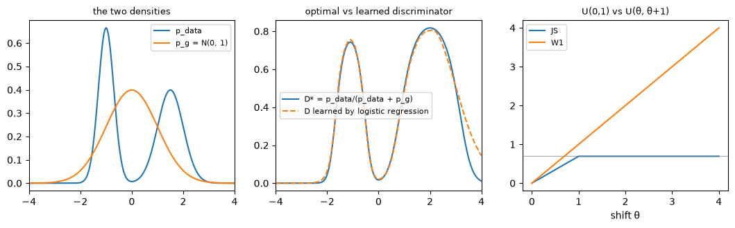
Code 01 uses 1-D distributions on a fine grid: and . A D trained only by logistic regression is compared with :
| quantity | value |
|---|---|
| max |D_learned − D*| where the data are | 0.038 |
| V(D*, G) by integration | −1.0368 |
| 2·JS − log 4 | −1.0368 |
| V(D_learned, G), Monte Carlo | −1.0385 |
The learned D lands on Bayes’ rule, and its value is just below the maximum, as any non-optimal D must be.
Moving toward the data:
| λ | JS | C(G) | E|D* − ½| |
|---|---|---|---|
| 0 | 0.1747 | −1.0368 | 0.244 |
| 0.5 | 0.0600 | −1.2663 | 0.122 |
| 0.9 | 0.0058 | −1.3748 | 0.024 |
| 1 | 0 | −1.3863 | 0 |
3.5 What the theory does not say
The theorems assume:
- D is optimal at every G-step. In practice it gets k gradient steps.
- G ranges over all distributions. In practice it is a network, and the parameters move, not itself.
- The game is solved in the order min over G of max over D. Alternating gradient steps do not respect that order; §4 shows what goes wrong.
The convergence statement in the paper, that converges to if D is optimal at each step and is updated directly, is about this idealized process. Lecture 11 returns to convergence with real parameterized models.
4. Problems of GANs
4.1 Three failure modes
The slides’ running example trains a GAN on MNIST. They show the D loss, the G loss and their real / fake parts over 500 epochs, with samples improving from noise to digits. Ideally the losses settle at the equilibrium values ( everywhere: D loss 2 log 2, G loss log 2). In practice the curves oscillate.
The slides list three problems:
- Hard to reach equilibrium. The two players chase each other; losses oscillate instead of converging.
- Vanishing gradients. If D becomes too good, its gradients for G vanish (§2.2 for the saturating loss; §5.1 for JS in general).
- Mode collapse. G produces only a few kinds of samples, each convincing.
Why does mode collapse happen? Take D fixed and do the G-step to completion. G is then rewarded for mapping every z to whatever x D currently finds most real, a single point. The alternating game only partly undoes this. D learns to reject the over-produced mode, G moves all of its mass to another one, and D follows. The theory’s min–max order would prevent this, since G would have to face the best response of D, but gradient steps play the game in both orders at once. Unrolled GANs (Metz et al., cited in the slides) let the G-step look ahead through several D-steps to approximate the right order.
4.2 Experiment: mode collapse and mode hopping on a ring
Code 02 trains the standard (non-saturating) GAN on 8 narrow Gaussians. Generated samples near each mode, out of 2000, every 1000 steps:
| step | m0 | m1 | m2 | m3 | m4 | m5 | m6 | m7 | covered | quality |
|---|---|---|---|---|---|---|---|---|---|---|
| 1000 | 42 | 653 | 243 | 33 | 18 | 19 | 25 | 24 | 2 | 0.53 |
| 3000 | 444 | 693 | 628 | 9 | 6 | 2 | 0 | 2 | 3 | 0.89 |
| 4000 | 30 | 1175 | 540 | 3 | 3 | 3 | 0 | 5 | 2 | 0.88 |
| 6000 | 614 | 545 | 500 | 8 | 1 | 155 | 1 | 1 | 4 | 0.91 |
| 8000 | 464 | 520 | 427 | 6 | 4 | 466 | 0 | 3 | 4 | 0.94 |
- Collapse. Never more than 4 of 8 modes.
- Hopping. Mode 0 is picked up (444), dropped (30), and picked up again (614): the oscillation of failure mode 1 made visible.
- Per-sample quality is excellent throughout (0.9). The failure is in the distribution, invisible to per-sample metrics.
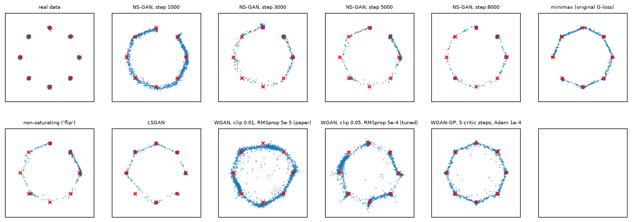
Five losses at the same budget (5000 G-steps; two seeds where shown):
| loss | modes covered | quality | mode entropy (max 3 bits) |
|---|---|---|---|
| minimax (original G-loss) | 7 / 8 | 0.81 / 0.88 | 2.85 / 2.99 |
| non-saturating (flip) | 3 / 3 | 0.86 / 0.89 | 1.36 / 1.68 |
| LSGAN (§5.6) | 7 / 8 | 0.94 / 0.94 | 2.78 / 2.99 |
| WGAN, clipping, paper settings (§5) | 3 | 0.17 | 2.45 |
| WGAN, clipping, tuned | 6 | 0.46 | 2.68 |
| WGAN-GP (§5.5) | 8 / 8 | 0.75 / 0.79 | 3.00 / 3.00 |
A surprise: the original minimax loss covered more modes than the flip trick on this toy. The flip fixes vanishing gradients early in training (§2.2), and the standard non-saturating GAN is not guaranteed to cover modes. GAN outcomes depend on the training dynamics, not only on where the equilibrium is. A plausible reason is that the minimax loss’s weak gradients for confidently rejected fakes make G react less violently to each D update. The losses designed around a better-behaved gap measure — LSGAN and WGAN-GP — were the most reliable.
4.3 Experiment: Problem Set 3 on glyphs
Problem Set 3’s architecture:
- G: z (64-d here) → 128 → 256 → 512 → image;
- D: image → 512 → 256 → 128 → 1, with dropout;
- LeakyReLU activations, no batch normalization.
Code 04 trains it on glyphs for 5000 G-steps (Adam 2e-4, β1 = 0.5, batch 64), with the three ablations and a conditional GAN:
| run (Problem Set 3) | valid | class H (bits) | FID | digits present |
|---|---|---|---|---|
| P1: baseline, seed 0 | 0.662 | 1.40 | 1716 | 5 |
| P1: baseline, seed 1 | 0.908 | 0.42 | 3507 | 2 |
| P1: baseline, seed 2 | 0.907 | 0.00 | 4450 | 1 |
| P2a: generator widths ×2 | 0.214 | 2.69 | 397 | 7 |
| P2b: deeper D (5 layers) | 0.695 | 1.52 | 2201 | 4 |
| P2c: 10 D-steps per G-step (2000 G-steps) | 0.100 | 1.45 | 907 | 5 |
| P3: conditional GAN | 0.560 | 3.32 | 23.5 | asked digit shown 98.6% |
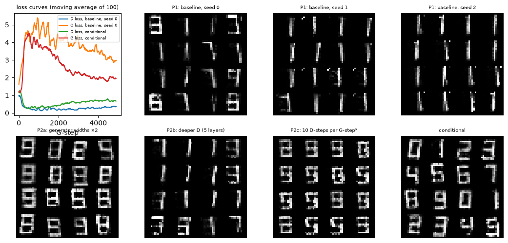
- Every unconditional run collapses. The glyphs are crisp and recognizable, but cover only a few digits; with seed 2, a single one. Eyeballing a 4×4 grid of samples, these runs look like successes. The Judge’s class entropy and FID expose them.
- None of the ablations fixes it. A larger G covers more digits (7) at much lower quality; a deeper D changes little. 10 D-steps per G-step gave poor samples after 2000 G-steps. In a 5000-step development run it reached valid 0.91 with about two digits — cleaner and even more collapsed.
- The conditional GAN works. G receives an embedded label concatenated with z, and D receives an embedded label concatenated with the image. Drawing the wrong digit is then punished, so the digit collapse is gone by construction, and the FID drops by two orders of magnitude. Lecture 6’s conditional PixelCNN showed the asked digit 32% of the time; this GAN 98.6%. Within a digit, z still changes the style.
Development note. LSGAN, the minimax loss and two more seeds also collapsed (class entropy 0–1.3 bits). WGAN-GP kept the diversity (2.94 bits) but had valid 0.02 after 5000 steps. On MNIST with many epochs the pset’s GAN works better; on our data, with this budget, conditioning is what makes it work.
5. Wasserstein GAN
The slides summarize WGAN in three registers (quoting a Reddit comment):
- for mathematicians: the Wasserstein distance instead of the JS divergence;
- for engineers: remove the logarithms, clip the weights;
- for laymen: an art critic instead of a forgery expert.
5.1 The problem with JS
If p and q do not overlap, then on the support of p, m = p/2, so KL(p ‖ m) = log 2; likewise for q. Hence , a constant, whatever the distance between them: no gradient.
The slides’ extreme case is two delta functions at 0 and θ: JS = log 2 for every θ ≠ 0 and 0 at θ = 0, a delta function of θ. A useful measure would grow smoothly with |θ|.
Code 01 (part 3) shifts U(θ, θ + 1) away from U(0, 1):
| θ | 0 | 0.25 | 0.5 | 1 | 1.5 | 2 | 4 |
|---|---|---|---|---|---|---|---|
| JS | 0 | 0.173 | 0.347 | 0.693 | 0.693 | 0.693 | 0.693 |
| W1 | 0 | 0.25 | 0.5 | 1 | 1.5 | 2 | 4 |
From θ = 1 on, JS cannot tell “slightly apart” from “far apart”. This is not a corner case: generated and real images occupy thin, low-dimensional sets in pixel space that typically do not overlap (Arjovsky & Bottou 2017). An optimal discriminator then separates them perfectly, and the G-gradient carries no information about where the data are.
5.2 The earth mover’s distance
Think of p as a pile of earth and q as a hole of the same volume. The 1-Wasserstein distance is the least total work (mass × distance) needed to move the pile into the hole.
1-D, discrete (the shovel example, after Lilian Weng). Piles P = (3, 2, 1, 4) and Q = (1, 2, 4, 3) on positions 1–4. Carry the surplus forward:
Here δ = (0, 2, 2, −1, 0), so W = 5 shovelfuls·steps. Code 03 solves the same problem as a linear program and gets 5 with the plan
from 1: 1 stays, 2 → position 2      from 2: 2 → position 3
from 3: 1 stays                       from 4: 1 → position 3, 3 stay
1-D, continuous. The running surplus is the difference of CDFs, so
For two deltas at 0 and θ, , exactly the smooth measure we wanted.
General. Over all couplings γ(x, y) whose marginals are p and q (transport plans: γ(x, y) is the mass moved from x to y),
5.3 Duality: from transport plans to critics (Problem Set 3, problem 5)
The infimum over couplings is intractable in high dimensions. Duality turns it into a supremum over functions — something a network can represent.
The discrete problem. Supplies and demands , both summing to 1, with a cost matrix C:
Deriving the dual. Introduce multipliers for the row constraints, for the column constraints, and for :
The dual function is unless every coefficient of vanishes, i.e. . Then
The requirement becomes . So the dual problem is
Weak duality (dual ≤ primal) holds by construction. For linear programs with a feasible primal (here is feasible) strong duality holds: the optimal values are equal. At the optimum, complementary slackness says .
Interpretation. A shipper charges to pick a unit of earth up at i and to drop it off at j. To stay competitive the charges can never exceed the cost of any route. The most the shipper can earn is exactly the cost of the best plan.
Checked in code 03. The transportation simplex (gan_tools.transport_simplex) solves the primal and produces the potentials (φ, ψ) as a by-product. On a random 4 × 5 problem:
| check | value |
|---|---|
| primal Σ T C | 3.988788 |
| dual Σ vφ + Σ wψ | 3.988788 |
| max (φ_i + ψ_j − C_ij) | 1.7e-16 |
| max |φ_i + ψ_j − C_ij| where T_ij > 0 | 1.7e-16 |
| Sinkhorn, ε = 1 / 0.3 / 0.1 | 4.178 / 4.043 / 3.997 |
| scipy linprog | 3.988788 |
Kantorovich–Rubinstein. When the cost is a distance, , the two potentials collapse into one function. Replace φ by its “c-transform” . This is a minimum of 1-Lipschitz functions, hence 1-Lipschitz, and one can show at the optimum. The dual becomes
where means : the slope is bounded by 1 everywhere. Code 03 builds this f from the simplex’s ψ on a 13-point grid:
- its Lipschitz constant is exactly 1.000;
- , equal to the OT cost and to the CDF formula;
- because p lies left of q everywhere, f is a straight line of slope −1. Where the CDFs cross, the slope would flip sign.
5.4 The WGAN objective
Replace the discriminator by a critic (no sigmoid, any real output) and keep it Lipschitz:
and train G to minimize it: maximize .
- Remove the logarithms. Compared with the original D-step, , the critic’s loss is linear in its outputs.
- Clip the weights. WGAN keeps the critic K-Lipschitz for some K by clipping every weight to [−0.01, 0.01] after each update. K is unknown, but scaling W1 does not change the direction G should move.
- Art critic, not forgery expert. The original D answers “real or fake?” — a probability that saturates. The critic gives a score (value, merit, quality) whose gradient points in the direction of improvement, even for samples far from the data.
The WGAN algorithm, as annotated in the slides: critic updates per G-update, RMSprop with learning rate 5e-5, clipping 0.01. The slides’ comparison shows WGAN producing usable samples where the original GAN’s training collapsed, and its loss correlating with sample quality, unlike the GAN loss.
5.5 Weight clipping vs a gradient penalty
Clipping is a crude Lipschitz control. Gulrajani et al. (2017, WGAN-GP; not in the slides) observed that it pushes critics toward simple, saturated functions and is sensitive to the clip value. They replaced it by a soft penalty at random points between real and fake samples, motivated by the fact that the optimal critic has slope 1 along the transport paths.
Code 03 (part 4) trains both critics between N(−1, 0.6²) and N(1.2, 0.9²), where the exact W1 = 2.200:
| critic | E_P f − E_Q f | max |f′| |
|---|---|---|
| weight clipping ±0.01 | 0.0077 | 0.004 |
| gradient penalty | 2.432 | 1.12 |
The clipped critic is a very weak function: Lipschitz constant 0.004, so it estimates 0.4% of W1. The GP critic is close, 10% above, because the soft penalty lets the slope exceed 1 a little. On the ring (§4.2), clipping with the paper’s settings covered 3 modes in 5000 steps, a tuned clip 6, and WGAN-GP all 8 in both seeds — at the highest cost per step (5 critic steps plus a double backpropagation).
5.6 Two more GAN losses (brief)
- LSGAN (Mao et al. 2017) replaces the log loss by least squares: D minimizes , and G minimizes . The penalty grows quadratically for fakes far on the “real” side of the decision boundary, so gradients do not vanish there. The paper shows this minimizes a Pearson χ² divergence for a suitable choice of targets. On our ring it covered 7–8 modes with the best quality (0.94).
- EBGAN (Zhao et al. 2017) views D as an energy function: low on real data, high elsewhere. D is an autoencoder whose reconstruction error is the energy, trained with a margin: . G minimizes the energy of its samples. Energy-based models return in Lecture 12.
6. The adversary as a loss function
6.1 The idea
The slides’ final part reframes the GAN. Its essence is an adversarial loss function:
- the generator’s input need not be random noise; it can be an image, a sketch, a low-resolution photo, a code;
- beyond L2 / L1, the adversarial loss encourages the output to look realistic;
- combined with L2 / L1, the reconstruction loss largely stabilizes training.
Pipeline: x → encoder → z → “decoder” → x′. The loss is plus an adversarial term from D. D is a parameterized loss function, trained alternately with the model.
6.2 Examples from the slides
| work | input → output | losses | lesson |
|---|---|---|---|
| SRGAN (Ledig et al. 2017) | low-res → high-res | content (MSE / VGG features) + adversarial | worse PSNR, better visual quality: L2 alone gives blurry textures |
| Context Encoder (Pathak et al. 2016) | image with a hole → filled hole | L2 + adversarial | L2 alone fills holes with blur |
| pix2pix (Isola et al. 2017) | image → image (edges → photo, maps ↔ aerial) | L1 + conditional GAN | a conditional D sees (input, output) pairs; a “PatchGAN” D judges local patches |
| CycleGAN (Zhu et al. 2017) | domain A ↔ domain B, unpaired | adversarial in both domains + cycle consistency ‖F(G(a)) − a‖ | the cycle loss replaces paired supervision |
6.3 From VQ-VAE to VQ-GAN
Lecture 3’s VQ-VAE trains its encoder–quantizer–decoder with L2 only, and its reconstructions are blurry. VQ-GAN (Esser et al. 2021) adds an adversarial loss (a patch discriminator) and a perceptual loss (distances between deep features). To be precise, as the slides say:
- VQ-GAN = VQ-VAE + adversarial loss + perceptual loss.
- Without the quantizer it is VAE + adversarial + perceptual loss.
- Both are the de facto tokenizers of image generation: with VQ for autoregressive models (Lecture 7), without VQ for latent diffusion models (Lecture 13). Commercial systems (Stable Diffusion, Sora) use such tokenizers.
The slides’ remark: “it involves everything” — an autoencoder (Lecture 3), quantization (Lecture 7), adversarial training (this lecture), and the generator built on top (Lectures 7, 8, 13).
6.4 Experiment: ghosts and bottlenecks
Completion (Lecture 1’s ghosts). Given the top half of a glyph, produce the bottom half. The tops of 2/3, 5/6 and 8/9 are identical. The discriminator always sees whole glyphs.
| completion model | pixel MSE | gray ink (real 0.091) | valid | FID | consistent (ambiguous tops) |
|---|---|---|---|---|---|
| L2 only | 0.0135 | 0.125 | 0.642 | 73.3 | 0.980 |
| L2 + adversarial | 0.0192 | 0.084 | 0.850 | 64.5 | 0.970 |
| adversarial only | 0.0393 | 0.080 | 0.685 | 62.9 | 0.854 |
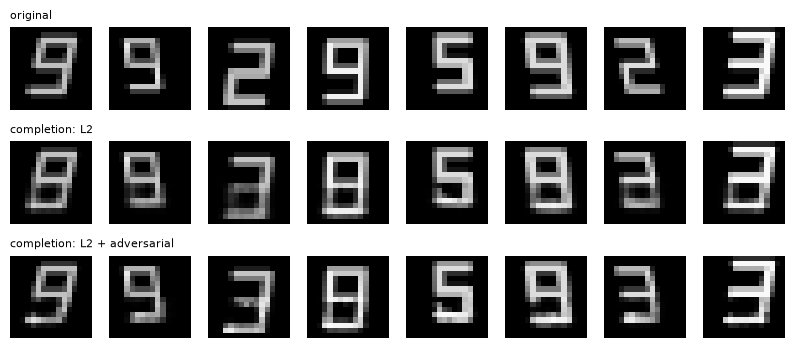
- L2 is “closest to the answer key” and least plausible. It averages the two possible bottoms of an ambiguous top, leaving half-transparent ghost ink.
- The adversarial term removes the ghosts by committing to one digit: higher pixel error, much higher valid rate. This is SRGAN’s trade-off in miniature.
- Adversarial alone follows the input less reliably. Nothing ties the output to the specific top except what D happens to check. The L2 term anchors; the adversary sharpens.
- With a noise input z, the same ambiguous top yields the other digit for 7% (λ = 1) or 23% (λ = 10) of new z. A regression task becomes a (weakly) generative one. pix2pix reported that its G learned to ignore the noise; with our strong adversary it uses it a little.
Reconstruction through a bottleneck (the VQ-GAN step). An MLP autoencoder with k numbers per glyph:
| autoencoder | RMSE | valid | FID | same digit as input |
|---|---|---|---|---|
| k = 4, L2 | 0.104 | 0.502 | 174.4 | 0.461 |
| k = 4, L2 + adversarial | 0.112 | 0.753 | 46.2 | 0.600 |
| k = 8, L2 | 0.039 | 0.989 | 2.2 | 1.000 |
| k = 8, L2 + adversarial | 0.043 | 0.980 | 2.4 | 1.000 |
- With a 4-number code, L2 cannot store every detail and outputs the average of what it cannot tell apart. The adversarial term trades a little RMSE for far better realism, and even keeps the digit right more often: a committed guess beats a blur that reads as nothing.
- With 8 numbers, the code suffices and the adversary adds nothing. Adversarial losses matter when the code is too small to describe the image. That is exactly the tokenizer regime: 256×256 images in a few hundred tokens.
7. The big picture
7.1 The five components of a GAN
| component | GAN |
|---|---|
| formulation | a latent-variable model , ; no density |
| representation | generator and discriminator networks |
| objective | a min–max game; at the optimal D, JS (original) or W1 (WGAN) between and |
| optimization | alternating gradient steps; the hardest part (equilibria, collapse) |
| inference | one forward pass per sample; no likelihood |
7.2 GANs among the families so far
| VAE | flow | autoregressive | GAN | |
|---|---|---|---|---|
| likelihood | lower bound | exact | exact | none |
| sampling cost | one pass | one pass | one pass per token | one pass |
| sharpness | blurry (per-pixel loss) | moderate | sharp | sharp |
| mode coverage | good | good | good | poor (collapse) |
| training | stable | stable | stable | unstable |
A GAN is the only family without a likelihood. That is its weakness (no direct measure of coverage, unstable training) and its strength (no per-pixel independence assumption, so sharp samples in one pass). Lectures 10–11 ask how far that strength scales, and whether the instability is inevitable.
8. Summary
- A network measures the gap. The discriminator replaces the reconstruction loss’s per-pixel independence assumptions with a learned real/fake classifier. The D-step is logistic regression; the G-step fools D. The flip trick gives G strong gradients early (10× in code 01).
- Theory. For a fixed G, D* = p_data/(p_data + p_g) (Bayes’ rule). Then V = 2·JS − log 4, minimized only at p_g = p_data. All three were confirmed numerically.
- Problems. Oscillation, vanishing gradients, mode collapse. On the ring the standard GAN never covered more than 4 of 8 modes and hopped between them. On glyphs, Problem Set 3’s GAN collapsed to 1–5 digits in every unconditional run, while its conditional version showed the asked digit 98.6% of the time.
- Wasserstein. JS is stuck at log 2 for non-overlapping distributions; W1 measures how far mass must move. Kantorovich duality (derived for the discrete case) turns W1 into a supremum over 1-Lipschitz critics. WGAN enforces the Lipschitz condition by clipping (weak, slow), WGAN-GP by a gradient penalty (robust, costlier).
- The adversary as a loss. With L2, an adversarial term trades pixel error for realism: ghosts disappear, and tight bottlenecks give readable reconstructions. This is the recipe of SRGAN, pix2pix and VQ-GAN, today’s standard tokenizer.
9. Common pitfalls
- “The GAN minimizes JS.” Only if D is optimal at every step; in practice it minimizes a moving, approximate target (§3.5).
- “Low D loss means a good model” / “the losses tell you the quality.” GAN losses oscillate around the equilibrium. Quality and coverage must be measured on samples, with metrics that see diversity (§4.3).
- “Crisp samples mean a good generator.” Mode collapse produces crisp samples of a few kinds (§4.2, §4.3).
- “The non-saturating loss is always better.” It fixes early vanishing gradients; it is not a mode-coverage guarantee (§4.2).
- “Weight clipping makes the critic 1-Lipschitz.” It makes it K-Lipschitz for an unknown, often tiny K (§5.5).
- “An adversarial loss is always an improvement.” It helps when the reconstruction is under-determined (ambiguity, tight bottlenecks); otherwise it adds instability for nothing (§6.4, k = 8).
- “WGAN’s critic outputs a probability.” It outputs an unbounded score; there is no sigmoid.
10. Exercises
Exercise 1 (Problem Set 3, 4a). Derive the optimal discriminator. What happens at x where , and where both are zero?
Answer
See §3.1: maximizing pointwise gives y = a/(a + b).
- Where : . D should be certain that x is fake.
- Where both are zero: x never appears in either expectation, so D(x) is arbitrary. This is why a learned D can do anything off the data (code 01: “Where neither distribution has mass, D is unconstrained”).
Exercise 2 (Problem Set 3, 4b). Show that and that its minimum −log 4 is attained iff .
Answer
See §3.2–3.3. A quick check of the value: at , and .
For the “only if”: , with equality iff both KL terms vanish. Since KL(p ‖ m) = 0 iff p = m, we need .
Exercise 3 (the flip trick, quantitatively). For : (a) show that the minimax and the non-saturating G-losses both decrease as the logit a of a fake sample increases, so they push G in the same direction; (b) compute the ratio of their gradient magnitudes as a function of D. Where are they equal?
Answer
(a) and : both losses fall as D(G(z)) rises. Neither derivative vanishes for finite a, so the G-loss alone has no stationary point; G’s equilibrium comes from D adapting (at , D can no longer raise or lower a).
(b) The ratio of magnitudes (non-saturating / minimax) is (1 − D)/D: 999 at D = 0.001, 1 at D = 0.5. They are equal at D = ½, which is where the equilibrium lies.
Exercise 4 (JS for non-overlapping supports). Prove that if p and q have disjoint supports, . Why does this imply that the optimal discriminator gives G no useful gradient?
Answer
On supp(p), q = 0, so m = p/2 and ; hence KL(p ‖ m) = log 2, and likewise KL(q ‖ m) = log 2. So JS = ½·log 2 + ½·log 2 = log 2.
For the second part: a small change of G that keeps the supports disjoint leaves JS unchanged, so the gradient of the ideal objective is zero. The optimal D is 1 on supp(p_data) and 0 on supp(p_g), and is flat (saturated) around the fakes, so the gradient through D is zero too. In practice D is not exactly optimal, and its gradients are uninformative rather than exactly zero.
Exercise 5 (Problem Set 3, 5c). Derive the dual of the discrete OT problem, and state complementary slackness. Verify it on the shovel example with : find potentials certifying that W = 5.
Answer
The derivation is in §5.3.
For the shovel example, the optimal plan uses the cells (1,1), (1,2), (2,3), (3,3), (4,3), (4,4). One certificate is φ = f(x), ψ = −f(y), with f 1-Lipschitz, slope −1 where mass flows right (positions 1–3, where the running surplus δ > 0) and slope +1 where it flows left (positions 3–4, δ < 0). Take f(1) = 0, f(2) = −1, f(3) = −2, f(4) = −1.
- Dual objective (with the unnormalized masses): Σ P_i f(i) − Σ Q_j f(j) = (3·0 + 2·(−1) + 1·(−2) + 4·(−1)) − (1·0 + 2·(−1) + 4·(−2) + 3·(−1)) = (−8) − (−13) = 5.
- Feasibility: f(i) − f(j) ≤ |i − j| holds because f is 1-Lipschitz.
- Tightness on the used cells: (1,2): 0 − (−1) = 1 ✓; (2,3): −1 − (−2) = 1 ✓; (4,3): −1 − (−2) = 1 ✓; the diagonal cells give 0 ✓.
Exercise 6 (W1 of Gaussians in 1-D). Show that for and , . Why is W1 between N(−1, 0.6²) and N(1.2, 0.9²) (code 03: 2.200) close to, but not exactly, 2.2 in general?
Answer
With equal σ, q is p shifted by Δ = μ₂ − μ₁. The map x ↦ x + Δ is a coupling moving every unit of mass by |Δ|, so W1 ≤ |Δ|. And for any coupling, . So W1 = |Δ|.
With different σ the quantile coupling moves the k-th quantile from μ₁ + σ₁z to μ₂ + σ₂z, so , Z ~ N(0, 1). This is ≥ |Δ|, with equality only when the sign of Δ + (σ₂ − σ₁)Z never flips. For Δ = 2.2 and σ₂ − σ₁ = 0.3, a flip needs Z < −7.3, so W1 = 2.2 to many digits — as code 03 found (2.2000).
Exercise 7 (why mode collapse). Consider a fixed D and a G-step taken to convergence with the non-saturating loss. What distribution does G produce? Why does alternating training not simply converge back to the data distribution?
Answer
The G-loss is . It is minimized by mapping every z to — a point mass, or a set of maximizers.
Alternating training then makes D lower its value there, and G moves its mass to the next maximum. The game is played as max–min rather than min–max: G responds to the current D instead of to D’s best response, so the process can cycle among modes rather than settle on covering all of them (code 02: mode hopping).
Fixes change the dynamics: unrolling D’s updates into the G-step, minibatch discrimination (D sees diversity), gradient penalties, or losses whose gradients keep pointing toward uncovered data (WGAN-GP).
Exercise 8 (hands-on).
(a) In 02_gan_2d.py, switch the data to the 5×5 grid (grid, GRID_CENTRES). Which losses cover all 25 modes?
(b) In 04_gan_glyphs.py, train the unconditional GAN with kind="wgan-gp" for 20,000 steps. Does quality catch up while diversity stays?
(c) In 05_adversarial_loss.py, replace the full-image discriminator by one that sees only the bottom half. What happens to “consistent”?
Answer (sketch)
(a) Expect the non-saturating GAN to cover a minority of modes and WGAN-GP / LSGAN most of them, at a lower quality on the grid’s outer modes. The grid is harder: many more modes for the same capacity.
(b) WGAN-GP keeps diversity because its critic’s gradients keep pointing at uncovered regions. Quality usually improves slowly, so expect a trend rather than parity within CPU budgets.
(c) A bottom-only D cannot check consistency with the top. The adversarial term then pushes toward any realistic bottom, the L2 term alone keeps consistency, and “consistent” should drop — more so for adversarial-only training.
11. Further reading
From the slides
- I. Goodfellow et al., Generative Adversarial Nets, NeurIPS 2014.
- M. Arjovsky, S. Chintala, L. Bottou, Wasserstein Generative Adversarial Networks, ICML 2017.
- M. Arjovsky, L. Bottou, Towards Principled Methods for Training Generative Adversarial Networks, ICLR 2017.
- L. Metz et al., Unrolled Generative Adversarial Networks, ICLR 2017.
- X. Mao et al., Least Squares Generative Adversarial Networks, ICCV 2017; J. Zhao, M. Mathieu, Y. LeCun, Energy-based Generative Adversarial Networks, ICLR 2017.
- C. Ledig et al., Photo-Realistic Single Image Super-Resolution Using a Generative Adversarial Network, CVPR 2017.
- D. Pathak et al., Context Encoders: Feature Learning by Inpainting, CVPR 2016.
- P. Isola et al., Image-to-Image Translation with Conditional Adversarial Networks, CVPR 2017.
- J.-Y. Zhu et al., Unpaired Image-to-Image Translation using Cycle-Consistent Adversarial Networks, ICCV 2017.
- P. Esser, R. Rombach, B. Ommer, Taming Transformers for High-Resolution Image Synthesis, CVPR 2021.
- L. Weng, From GAN to WGAN, arXiv:1904.08994 (blog post; the shovel figures).
- Interactive: GAN Lab, https://poloclub.github.io/ganlab/.
Beyond the slides
- I. Gulrajani et al., Improved Training of Wasserstein GANs (WGAN-GP), NeurIPS 2017.
- M. Cuturi, Sinkhorn Distances: Lightspeed Computation of Optimal Transport, NeurIPS 2013.
- G. Peyré, M. Cuturi, Computational Optimal Transport, 2019 (chapters 2–3: the discrete problem and its dual).
- I. Goodfellow, NIPS 2016 Tutorial: Generative Adversarial Networks (mode collapse and the min–max order).
Related notes in this course
- Lecture 1 §2–3 (ghosts; discriminative vs generative and Bayes’ rule).
- Lecture 3 §7 (VQ-VAE, the tokenizer VQ-GAN improves).
- P1 (KL divergence; forward vs reverse KL).
12. Next lecture
Lecture 10: Scaling GANs — text-to-image and distillation (reading session · 10/08).
By 2022, diffusion models had taken over text-to-image generation. Their samples are better and their training more stable, but they need many network passes per image. GANs still have their great advantage: one pass. Lecture 10’s papers ask whether GANs can be scaled to large text-to-image models after all:
- StyleGAN-T and GigaGAN redesign generators and discriminators for text conditioning and billions of images;
- Diffusion2GAN distills a slow diffusion model into a one-step conditional GAN, using regression plus an adversarial loss — the combination we just saw remove ghosts.