Maps to: MIT 6.S978 Deep Generative Models (Fall 2024, MIT EECS; taught by Kaiming He, TA Minghao Guo), Lecture 1 · Thu 09/05/2024 · Introduction. Reading: Lecture 1 slides (
lec1_intro.pdf, course page https://mit-6s978.github.io/). The works cited on the slides are listed in §12. Basis: This lecture follows the Lecture 1 slides:
- examples from the GenAI era and its prehistory (Efros–Leung texture synthesis, PatchMatch);
- what generative problems have in common;
- discriminative vs generative models and Bayes’ rule;
- where probability comes from (latents and world models, probability as part of the modeling, underfitting and overfitting);
- generative models with probabilistic modeling;
- the five components of deep generative models;
- writing real problems as .
The slides give only these points and figures. These notes add the mathematics behind them — the optimum of squared error, the two directions of Bayes’ rule, KL and maximum likelihood, forward vs reverse KL, conditional entropy — and all the experiments. GlyphWorld and every toy experiment were designed for these notes and do not reflect what was said in class. Code:
code/lecture01/(7 scripts + 3 modules; numpy + PyTorch (CPU) + matplotlib; 1–10 seconds each) Reading time: 4–5 hours including running the code
0. How to read this lecture
0.1 Learning goals
After this lecture you should be able to:
- Name what problems “needing a generative model” have in common (one-to-many, some answers more plausible than others, no exact answer in the training data, output more complex than input), and explain why regression (minimizing squared error) on such problems yields “the average of all answers” — an answer that often looks like none of them.
- Distinguish discriminative models from generative models , move between them with Bayes’ rule, and say exactly “what a discriminative model is missing to become a generative one”.
- Explain where the probability of data comes from with “latents + a world model”: why simple latents passed through a deterministic map produce a complex data distribution, and why fitting simple models directly in pixel space fails.
- Understand that “probability is part of the modeling”: we only have finitely many samples and the model must extrapolate; recognize underfitting and overfitting in generative models, and know that “a δ function on every training point” means memorizing the training set.
- Derive “maximizing likelihood = minimizing the KL divergence”, and understand the two different errors (“blur” vs “miss”) that forward and reverse KL produce when the model family is too small.
- Name the five components of a deep generative model (formulation, representation, objective, optimization, inference), and point out which parts are “designed” and which are “learned” in autoregressive and diffusion models.
- Write chat, text-to-image, class-conditional generation, classification and robot policies as , and use conditional entropy to understand “the more abstract , the more generative the problem”.
0.2 Prerequisites and scope
The original course requires a deep-learning course (MIT 6.S898 / 6.7960) plus either computer vision or NLP. This lecture is the map of the whole course and needs very little mathematics:
| Assumed | Previewed only (developed later) |
|---|---|
| probability densities, expectations, conditional probability, Bayes’ rule (read prerequisite P1 first if unfamiliar) | VAEs and the ELBO (Lecture 3); normalizing flows (Lecture 4) |
| means, variances; 1-D and multivariate Gaussians | network architectures and training of autoregressive models (Lectures 5–8) |
| a little Python; a rough idea of what “training a neural network” means | GAN minimax and the JS divergence (Lecture 9) |
| logs, sums, derivatives | diffusion models, score matching, flow matching (Lectures 12–18) |
0.3 Map
§1  the "GenAI era" and its prehistory: Efros-Leung texture synthesis, PatchMatch
§2  which problems need generative models: one-to-many; regression averages; "ghosts"        ← code 01
§3  discriminative vs generative: the two directions of Bayes' rule; "the most-8-like image"  ← code 02
§4  where probability comes from: latents and world models; finite data; under/overfitting   ← code 03, 04
§5  generative models with probabilistic modeling: KL and maximum likelihood; forward vs reverse KL ← code 05
§6  deep generative models: representing distributions; designed vs learned; five components ← code 06
§7  writing real problems as p(x|y): cases and conditional entropy                              ← code 07
§8  the big picture: what this course covers
§9  summary   §10 common pitfalls   §11 exercises   §12 further reading   §13 next lecture
Suggested order: §1 → §2 → run 01 → §3 → run 02 → §4 → run 03, 04 → §5 → run 05 → §6 → run 06 → §7 → run 07 → §8.
0.4 Notation (used throughout the course)
| Symbol | Meaning |
|---|---|
| “data”: what we want to generate (a flattened image, a reply, a 3-D structure, a sequence of actions) | |
| condition: a prompt, a class, an observed part, a constraint, … (§7: “more abstract, less information”) | |
| latent variable: factors not directly observed but that “decide what the data look like” (pose, lighting, font, …) | |
| the data distribution: we only see it through samples and never get its formula | |
| the model distribution; are learnable parameters (usually network weights) | |
| expectation: the average of when is drawn from | |
| KL divergence (§5): | |
| , | entropy, conditional entropy (§5, §7), in bits (base 2) or nats (base e), stated each time |
0.5 About 6.S978
6.S978 is a graduate seminar taught by Kaiming He in MIT EECS (“S” marks a special-topics course; these notes follow the Fall 2024 edition). He was previously at Facebook AI Research. He is best known for ResNet, Faster / Mask R-CNN, MoCo and MAE — all “discriminative” or “representation-learning” work. In recent years his research has turned to generative models; for example, MAR, which appears as an example on the slides, is covered in Lecture 8. The course description focuses on computer vision (images, video, geometry), with related fields such as robotics, biology and materials.
The format of the course determines how these notes are written:
- 5 lectures: introduction (this one), VAE, autoregressive models, GANs, energy-based models / score matching / diffusion. Kaiming He teaches the core modeling idea of each family, not the latest tricks.
- 17 paper-reading sessions: 3 papers each, with 20-minute student presentations. The papers range from 1999 texture synthesis to Movie Gen and AlphaFold 3 in 2024.
- 2 guest lectures: Jun-Yan Zhu (data ownership) and Yang Song (consistency models).
- 6 problem sets: VAE, PixelCNN, GAN, DDPM, conditional flow matching, consistency models — all on MNIST.
The last slide says the course covers three things:
- how real-world problems are formulated as generative models;
- probabilistic foundations and learning algorithms;
- challenges, opportunities and open problems.
Note the first one: “how to formulate a problem as a generative model” (formulation) comes first. This perspective runs through the whole course. The same problem can be modeled in many ways, and which one you pick often matters more than which network architecture you use.
0.6 The toy worlds
Real image distributions have no formula, so the code of these notes uses two kinds of data “made by code, with the truth fully known”:
(1) The seven-segment digit world (GlyphWorld, toy_worlds.py). Every image has 16×16 = 256 pixels with gray levels in . An image is generated in two steps:
- Draw 7 latents (“knobs”): the digit class (uniform over 0–9), horizontal shift dx, vertical shift dy, size scale, slant, stroke thickness thick, ink intensity ink — each continuous knob uniform on an interval.
- Hand them to a deterministic renderer of a few dozen lines: light up segments by the seven-segment rules; the closer a pixel is to the nearest lit segment, the brighter it is (with a 1-pixel soft edge).
      a          0: abcdef   1: bc     2: abdeg   3: abcdg   4: bcfg
    ─────        5: acdfg    6: acdefg 7: abc     8: abcdefg 9: abcdfg
 f │     │ b
   │  g  │
    ─────
 e │     │ c
   │     │
    ─────
      d
This is a concrete instance of the “latents → world model → observation” of §4. Because the generating process is known, many quantities that are usually impossible to compute become exact:
- how many possibilities the other half of an image has, given one half;
- whether a generated image is “valid” (read whether each segment is lit, and see whether they spell a digit);
- conditional entropies under various conditions.
The code of the whole course uses it in place of MNIST.
(2) Known 1-D / 2-D distributions: Gaussian mixtures (with a density formula) and a 2-D “sine-wave band”. They demonstrate concepts that need exact densities, such as density estimation and the KL divergence.
1. The “GenAI” era and before
1.1 What today’s generative models do
The slides open with six examples:
| Application | Example | Input → output |
|---|---|---|
| chat and natural-language dialogue | ChatGPT-style chatbots | a prompt → a reply |
| text-to-image | Stable Diffusion 3 Medium drawing “a teddy bear teacher writing generative models on a blackboard” | a sentence → an image |
| text-to-video | Sora | a sentence → a video |
| code generation | AI coding assistants | comments / context → code |
| protein design and generation | RFdiffusion (Watson et al., Nature 2023) | constraints → a 3-D structure |
| weather forecasting | precipitation nowcasting with deep generative models (Ravuri et al., Nature 2021) | past radar maps → future radar maps |
These applications span text, images, video, code, molecules and weather, and seem to have nothing in common. §2 explains why they all need “generative models” rather than the familiar “classification / regression models”.
1.2 Prehistory I: texture synthesis in 1999 (Efros–Leung)
Generative models did not appear in the 2020s. The slides deliberately show two “pre-GenAI” examples. The first is the texture synthesis algorithm of Efros and Leung (1999) (Texture Synthesis by Non-parametric Sampling, ICCV 1999).
The problem: given a small piece of texture (a brick wall, a piece of fabric), generate a large new image that “looks like the same texture but is not a simple copy-paste”.
Their method is strikingly simple:
- Start from a small seed (a piece cut from the example) and grow outward one pixel at a time.
- To fill a new pixel, look at its already filled neighbours, forming a “small window with holes”.
- Find all locations in the example texture whose windows are “similar enough” (within a factor of the best match’s distance).
- Pick one of these locations at random and copy its center pixel.
The random pick in step 4 is crucial:
- always picking the best match makes the texture fall into an endless loop repeating the same fragment;
- averaging the center pixels of all matches makes the texture blurrier and blurrier.
Picking one at random is sampling from “the conditional distribution of the center pixel given its neighbours”. That conditional distribution has no formula; it is represented “non-parametrically” by the matching locations in the example.
The slides’ verdict: “in today’s language, this is an autoregressive model.” Indeed:
- it generates one element after another in some order (“auto”: it uses what it has generated as input);
- each step samples from a conditional distribution ;
- only the conditional distribution is not given by a neural network but estimated by “finding neighbours in the example”.
Twenty-odd years later, GPT generating text and the early PixelCNN generating images use exactly the same skeleton, with “finding neighbours in the example” replaced by “predicting the conditional distribution with a neural network”. Part 2 of script 01 implements an Efros–Leung-style “nearest-neighbour sampling”, and you will see the difference between “sampling” and “averaging” with your own eyes.
1.3 Prehistory II: PatchMatch in 2009 (content-aware fill)
The second example is PatchMatch (Barnes et al., SIGGRAPH 2009), which became the core algorithm behind Photoshop’s “Content-Aware Fill”: circle a person or a telephone pole in a photo, and the software fills the hole with plausible surrounding content.
PatchMatch itself is a fast randomized algorithm for approximate nearest neighbours: for every small patch of an image, find the most similar patch elsewhere. Brute force is too slow. PatchMatch’s insight is that natural images are highly coherent: if a patch has found a good match somewhere, its right-hand neighbour can probably find a good match just to the right of that location. So the algorithm alternates two steps:
- propagation: try “borrowing” the good matches found by neighbours;
- random search: try a few random locations around the current match, with exponentially shrinking radius.
A few iterations converge to very good results.
Like Efros–Leung, PatchMatch’s “generative” ability comes from finding suitable fragments in existing data and stitching them together. It has no explicit probability model, yet it solves an essentially generative problem: “what should be in this hole?” — the answer is not unique; it only has to be plausible.
1.4 Why start from “old methods”
These two examples hint at an undercurrent of the course: many core ideas of today’s deep generative models appeared before deep learning:
- sampling element by element from conditional distributions (autoregression);
- defining distributions by the data themselves (non-parametric methods);
- outputs that are “plausible” rather than “correct”.
What deep learning brings is representational power. Conditional distributions that used to be represented by “finding neighbours in the example” are now represented by neural networks, which generalize to combinations never seen in the training data. The Lecture 2 reading session is devoted to the “image priors” of the pre-deep-learning era.
2. What problems need generative models
2.1 Four common features
The slides ask: what do chatbots, image generation, video generation and protein generation have in common? Four things:
- One input corresponds to multiple, even infinitely many, predictions. “Draw a cat” can be drawn as countless different cats; “hello” has countless appropriate replies.
- Some predictions are more “plausible” than others. A five-legged cat is a “possible” output but far less plausible than a normal cat.
- The training data may contain no exact answer at all. The training set has no image of “a teddy bear wearing an astronaut helmet riding a horse”; the model must compose something new.
- The prediction is often more complex, more informative and higher-dimensional than the input. A prompt of a dozen words must produce an image with a million pixels.
Compare the familiar discriminative task of image classification: the input is an image, the output one label, “dog”. There is a single “desired output”, and the output (1 of 10 or 1 of 1000) is far simpler than the input (hundreds of thousands of pixels). The discriminative mindset is “for every input, find the correct answer”. A generative task asks instead “for every input, give a distribution and sample from it”.
2.2 A minimal example: given , guess
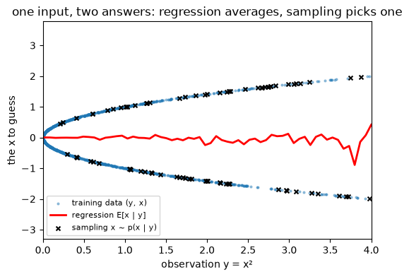
Start with the simplest case (part 1 of script 01). is standard normal; we only see and must guess . Every obviously has two equally plausible answers, and .
What does the discriminative habit — train a regression model minimizing the squared error — give? The experiment (20,000 training samples, binned by ):
| interval of | plausible | regression | sampling (6 draws) |
|---|---|---|---|
| [0.25, 0.50) | ±0.50 to ±0.71 | −0.008 | −0.61 −0.69 −0.58 −0.69 +0.60 −0.63 |
| [0.50, 1.00) | ±0.71 to ±1.00 | +0.009 | −0.96 +0.74 +0.96 +0.94 +0.73 +1.00 |
| [1.00, 2.00) | ±1.00 to ±1.41 | −0.040 | −1.40 −1.37 +1.21 +1.17 +1.37 +1.22 |
| [2.00, 4.00) | ±1.41 to ±2.00 | −0.062 | −1.83 +1.67 −1.47 −1.45 +1.83 +1.73 |
The regression answers are almost all 0 — the average of the two answers. But : for every , the regression answer is an “impossible” . On 1500 test points we measure “plausible” (the absolute value of the prediction within 0.1 of ):
- regression is plausible 0.0% of the time;
- sampling is plausible 99.7% of the time, and gives a positive sign 47.3% of the time — about half each.
2.3 Why regression must “average”
This is not a badly trained regression model; it is dictated by the squared-error objective itself. Let be the quantity to predict and the input. For any predictor :
After expanding the square, the cross term is 0: first take the expectation over given , and the conditional expectation of the first bracket is 0. The first term does not depend on , and the second is minimized (to 0) by . Therefore:
The squared-error-optimal prediction is the conditional expectation — the probability-weighted average of all plausible answers.
When the conditional distribution has a single sharp peak, the average sits on the peak and regression works well. When has several peaks, the average falls between them — somewhere that looks like none of them. This is the direct consequence of feature 1 of generative problems (one-to-many).
2.4 Experiment: completing glyphs, and “ghosts”
Now the same phenomenon in images (part 2 of script 01). Given only the top half of a glyph (rows 0–7), complete the bottom half. The key: 2 and 3, 5 and 6, 8 and 9 have identical top halves — one input, two plausible answers. Five completion methods are compared:
- (A) Oracle regression : use knowledge of the true world to compute the bottom halves of the two candidate digits and average them. Squared-error optimal; unavailable in reality.
- (B) MLP regression: an ordinary neural network, input the top half, output the bottom half, trained with squared error on 20,000 training images.
- (C) Nearest-neighbour average: find the 5 training images with the most similar top halves and average their bottom halves.
- (D) Nearest-neighbour sampling: the same 5 neighbours, pick one at random and copy its bottom half — the Efros–Leung idea.
- (E) Oracle sampling: pick one of the two candidates with probability 1/2 each and draw it in the true style.
Three rulers grade them:
- per-pixel squared error;
- crisp: the three bottom segments c, d, e are each either lit or dark, without half-transparent ghosts;
- valid: top and bottom together read as some digit 0–9.
On the 622 test images with ambiguous top halves:
| completion method | squared error | crisp | valid | original digit guessed |
|---|---|---|---|---|
| (A) oracle regression | 0.0073 | 0.0% | 0.0% | 0.0% |
| (B) MLP regression | 0.0088 | 0.2% | 0.2% | 0.0% |
| (C) nearest-neighbour average | 0.0130 | 24.6% | 24.6% | 12.1% |
| (D) nearest-neighbour sampling | 0.0248 | 85.5% | 85.2% | 40.2% |
| (E) oracle sampling | 0.0152 | 100.0% | 100.0% | 47.4% |
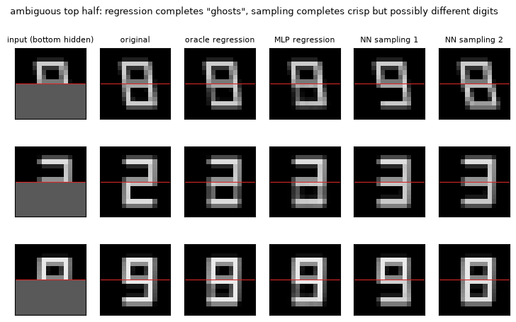
The figure shows it most clearly. When the original is an 8, regression draws a half-transparent “ghost” where the lower-left segment e should be: the average of an 8 (e lit) and a 9 (e dark). The MLP learns almost exactly the oracle regression (squared error 0.0088 vs 0.0073): the neural network is not wrong; it faithfully learned what you asked it to learn — the conditional expectation. Sampling completes a crisp 8 or 9. About half the time it “guesses wrong” about the original digit, but that “wrong” answer is just as plausible: the top half alone cannot distinguish 8 from 9.
On the 378 unambiguous test images (0, 1, 4, 7), MLP regression is crisp and valid 98.9% of the time: when an input has only one answer, regression is enough and no generative model is needed.
In the real world this “ghost” phenomenon is called blurriness. Image prediction, super-resolution and video prediction trained with an L2 loss are always blurry, precisely because of the averaging seen here. Later lectures connect back to it: VAE samples are blurry (Lecture 3), and GANs introduce an adversarial loss to “de-blur” (Lecture 9).
2.5 Why per-pixel error is a bad ruler
The table holds another intriguing number. Oracle sampling has a higher squared error (0.0152) than oracle regression (0.0073), with a ratio of 2.09. The “about 2×” is no coincidence. Let be the true bottom half, an independent draw from the same conditional distribution, and :
(The cross term vanishes because and are independent with mean .) The right-hand is exactly the squared error of oracle regression. So:
A perfect generative model has exactly twice the per-pixel squared error of a perfect regression model.
Ranking generative models by squared error (or the equivalent PSNR) systematically favours “blurry” answers. That is why generative models need other evaluations:
- likelihood (§5);
- distances between the sample distribution and the real distribution (FID-type metrics, prerequisite P2);
- human preference studies.
2.6 Copying nearest neighbours: how much data is enough?
Nearest-neighbour sampling (D) is only 85.5% crisp on ambiguous inputs, not 100%. Why? Because it can only copy. No training image has exactly the style (position, thickness, slant, …) of the test image, so the copied bottom half does not line up with the visible top half, and the segment reader lands on “half-lit” positions. Part 3 of script 01 varies the training-set size:
| training-set size | distance of the nearest neighbour | completion squared error | crisp | valid |
|---|---|---|---|---|
| 2,000 | 0.0619 | 0.0279 | 66.9% | 64.0% |
| 6,000 | 0.0493 | 0.0219 | 78.5% | 77.5% |
| 20,000 | 0.0390 | 0.0168 | 89.2% | 88.7% |
| 60,000 | 0.0321 | 0.0155 | 95.2% | 95.1% |
More data means a more similar nearest image and better results, but the growth is slow: a 30× larger training set only halves the nearest-neighbour distance. Here there are only 6 continuous style factors. Real images have far more “style” dimensions, and copying would need impossibly much data.
This is what feature 3 of generative problems (no exact answer in the training data) means: the model must interpolate between training samples and compose new things. Non-parametric copying cannot do that, so we need parametric models that generalize — neural networks.
But Efros–Leung’s idea still stands: for one-to-many problems, draw one from the conditional distribution instead of averaging.
2.7 Summary
The essence of a generative problem: for one input, there is a distribution of plausible answers. Regression (minimizing squared error) gives the mean of that distribution, which looks like nothing when there are several peaks; a generative model must represent the distribution and sample from it. Per-pixel error favours the mean and cannot evaluate generation.
3. Discriminative vs. generative models
3.1 Two directions
The slides draw the two kinds of models as arrows in two directions:
- Discriminative model: input a “sample” (an image), output a “label” (“dog”). It learns ; for every input, one desired output.
- Generative model: input a “label” (“dog”), output a “sample” (an image of a dog). It learns ; for every input, many possible outputs.
The meanings of and do not change: is always “data / sample”, always “label / condition”. What changes is the direction of the arrow.
3.2 A generative model can be used as a discriminative one: Bayes’ rule
Given a generative model and the prior (how common each class is), Bayes’ rule immediately gives a discriminative model:
The slides point out that the denominator “is a constant for a given ”: to classify, we only compare across , without computing . So “a generative model can be discriminative” (given the prior).
3.3 Can a discriminative model be used as a generative one? It needs
In the other direction, with a discriminative model we want :
This time the denominator is a constant for a given , no problem. The trouble is the extra in the numerator — the distribution of the data itself, which a discriminative model never models. The slides conclude: “for a discriminative model to become generative, one still needs to model the prior distribution of .” And (“the distribution of all natural images”) is exactly the hardest thing to model. Hence:
The challenge is about representing and predicting distributions.
Neither direction escapes “representing a distribution”: a generative model must represent , and a discriminative model that wants to generate must supply .
3.4 Experiment: one dataset, two classifiers
Script 02 compares two classifiers in a 2-D two-class world (each class a Gaussian; during training ):
- Generative classifier: fit a Gaussian per class (sample mean, sample covariance) plus the class frequencies , and classify with Bayes’ rule (in statistics, quadratic discriminant analysis, QDA).
- Discriminative classifier: logistic regression fitting directly, with quadratic features so that both decision boundaries belong to the same family.
| classifier | accuracy | log loss |
|---|---|---|
| generative (fit and , Bayes’ rule) | 0.9073 | 0.2141 |
| discriminative (fit directly) | 0.9076 | 0.2161 |
| Bayes optimal (true parameters) | 0.9088 | 0.2121 |
The two routes almost tie. The generative one has a slightly lower log loss here because its assumption (each class is Gaussian) happens to be true. On real data the discriminative one usually wins: “getting the distribution of right” is much harder than “only getting the boundary right”, and a discriminative model only needs the latter. This also explains why the first decade of deep learning was dominated by discriminative models.
What if the prior changes? At test time the class proportion changes from 0.3 to 0.8:
| classifier | accuracy | log loss |
|---|---|---|
| generative, still with the old prior | 0.8471 | 0.3643 |
| generative, with the new prior 0.8 | 0.9411 | 0.1633 |
| discriminative, used as is | 0.8553 | 0.3691 |
| discriminative + correction | 0.9401 | 0.1676 |
| Bayes optimal (new prior) | 0.9418 | 0.1625 |
The generative classifier only needs to swap to almost match the Bayes optimum, because it models “what looks like within each class” and “how common each class is” separately. The discriminative one can be corrected too, but the correction itself is derived from Bayes’ rule and quietly uses the generative view that ” does not change”.
3.5 Experiment: “generating” with a discriminative model
Next we try (part 3 of script 02), comparing three sources:
| source | mean | std | in the 95% high-density region of the true |
|---|---|---|---|
| true | (+1.22, +0.79) | (0.77, 1.11) | 95.0% |
| (a) discriminative × true (unlabeled samples reweighted by ) | (+1.24, +0.83) | (0.77, 1.11) | 95.1% |
| (b) discriminative × uniform “prior” (no ) | (+1.64, +0.39) | (3.86, 4.93) | 9.6% |
| (c) sample the generative model directly | (+1.25, +0.81) | (0.78, 1.04) | 95.5% |
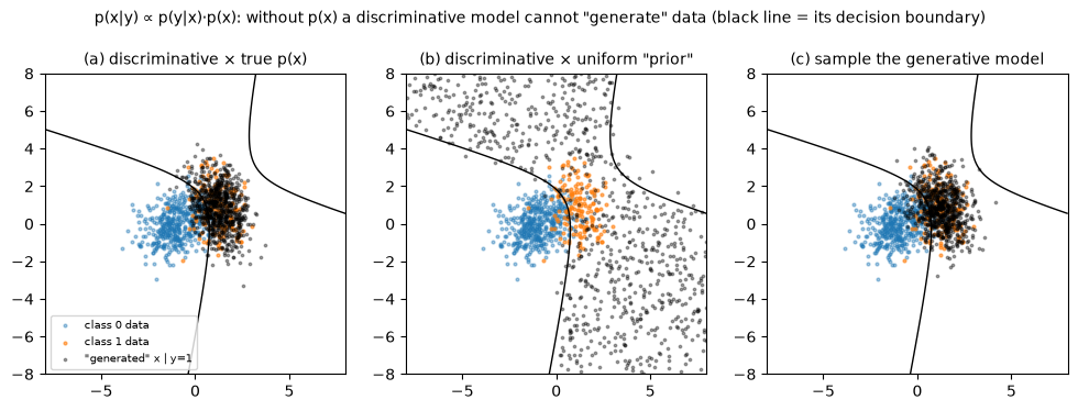
(a) shows that the formula is right: given (here a large pool of unlabeled samples), reweighting yields the correct conditional distribution. (b) is what happens “without ”. A discriminative model only knows “which side of the decision boundary is class 1”, so the points “most like class 1” spread over the whole half plane, and 90% land where real data never appear.
“The most-8-like image” (part 4 of script 02) applies the same idea to images. Train a digit classifier on GlyphWorld (test accuracy 100%) and ask it “what does the most 8-like image look like to you?” Starting from an all-gray image, run gradient ascent on the input pixels to maximize .
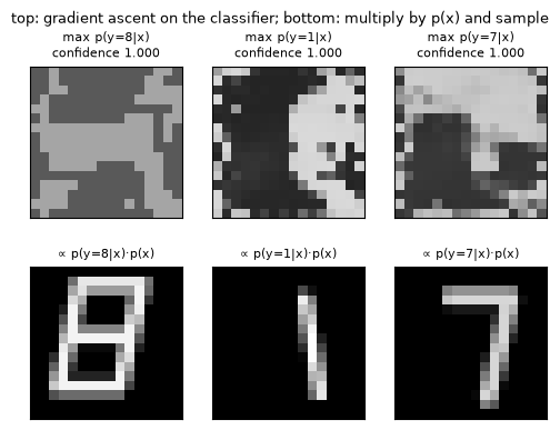
The classifier is 1.0000 confident about all three images, yet they are not digits at all. They lie 0.418, 0.457 and 0.489 from the nearest real image, 6–8 times the distance of real test images (0.064). A discriminative model learns “the boundary between 8 and the other digits”; maximizing finds the most extreme point on the far side of the boundary, not a typical 8 — a close relative of “adversarial examples”. Multiply in (a pool of real images) and sample , and real 8, 1 and 7 appear at once (bottom row).
3.6 Summary
Generative model + prior → discriminative model (Bayes’ rule); discriminative model + → generative model. Both directions need to represent a distribution, and the distribution of high-dimensional data is the hardest part. This is the central problem of the course.
4. Where does probability come from?
4.1 Latent variables and “world models”
We keep saying “the data distribution ”, but why would a photo have a “probability”? The slides’ first answer: assume the data are produced by some generative process.
- There are latent factors : an object’s pose, lighting, size, …
- follows a simple distribution (e.g. independent uniform or Gaussian factors).
- The observation is rendered by a “world model”: , where is a function of (physics, imaging, a renderer, …).
- So has a complex distribution.
The slides’ figure comes from Freeman and Tenenbaum’s bilinear models (Learning Bilinear Models for Two-Factor Problems in Vision). The same letter (“content”) written in different fonts (“style”), or the same face photographed under different lighting, can be described as a bilinear combination “style factor × content factor”. It is an early representative of the idea of “decomposing observations into a few simple factors”.
So the slides say: probability is part of the modeling. “The data follow some distribution” is itself a modeling assumption we make. The assumption is useful because it lets us talk about “which data are more common, more plausible”.
4.2 Experiment: simple , complex
GlyphWorld is exactly such a “latents + world model” (script 03). All 7 latents are uniform:
| latent | distribution |
|---|---|
| digit class | uniform on {0, …, 9} |
| dx, dy (shift) | U[−1.5, 1.5], U[−1.2, 1.2] pixels |
| scale (size) | U[0.85, 1.10] |
| slant | U[−0.25, 0.25] |
| thick (stroke half-width) | U[0.55, 0.95] pixels |
| ink (intensity) | U[0.75, 1.00] |
After the renderer, the distribution of the 256 pixels becomes quite complex:
-
Single pixels look like no simple distribution. 74.0% of pixel values are exactly 0 (pure background). A particular pixel (row 3, column 8) is 0 28.7% of the time, above 0.6 37.1% of the time, and in between otherwise — a mixture of “a big lump at 0 + a spread of bright values”.
-
Pixels have long-range dependencies. Neighbouring pixels have a mean absolute correlation of 0.475, and pixels 12 apart still 0.118. Two concrete examples:
- two pixels at the ends of the top bar a (5 columns apart) have correlation +0.771: the same stroke lights up together;
- two pixels on the left and right of the same row (8 columns apart) have −0.499: an overall shift makes the left bright when the right is dark.
These long-range dependencies come from “one set of latents controlling all pixels at once”.
-
The data lie on a curved, low-dimensional “surface”. Principal component analysis (PCA) needs 16 / 27 / 41 / 84 directions to explain 80% / 90% / 95% / 99% of the pixel variance, while these images were generated with only 7 knobs. The set the data occupy (a manifold) is 7-dimensional, but curved, and enclosing it in a flat subspace takes dozens of dimensions. The complexity of “simple → complex” comes from the nonlinearity of the renderer.
4.3 What if we fit simple models directly in pixel space?
The data distribution is complex — can we ignore the latents and fit a simple model directly in pixel space? Part 3 of script 03 tries three. It measures realism by “the per-pixel RMS distance to the most similar of 20,000 real images”: fresh real images give about 0.066 (the “floor”), pure random noise about 0.49.
| how generated | nearest-real distance (median) | fraction with distance < 0.1 |
|---|---|---|
| (i) independent pixels (each pixel’s marginal exactly right) | 0.244 | 0.0% |
| (ii) one 256-dim Gaussian (mean + full covariance) | 0.157 | 0.2% |
| (iii) one Gaussian per digit (10 components, true labels) | 0.135 | 13.6% |
| (iv) latents + world model (the true distribution) | 0.066 | 95.2% |
| reference: uniform random noise | 0.490 | 0.0% |
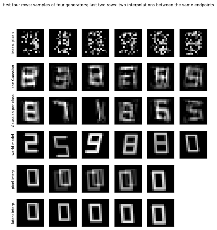
- (i) Every pixel’s distribution is right, yet together they form random speckle: all dependencies between pixels are lost.
- (ii) One big Gaussian captures “pairwise linear correlations”; its samples are a faint “superposition of all digits”.
- (iii) Knowing the digit, an outline appears, but the strokes are blurry and speckled.
- (iv) Only simple latents plus a nonlinear map produce real digits.
An interpolation experiment shows further what “latent space” means. Take two images , of the same digit in two styles:
| interpolation | nearest-real distance (median, 300 pairs) |
|---|---|
| endpoints (real images) | 0.063 |
| pixel-space midpoint | 0.105 |
| latent-space midpoint | 0.060 |
The average of two plausible images in pixel space is often not a plausible image: two offset digits superimpose into a “double image” (second-to-last row of the figure). Averaging in latent space and then rendering gives a digit “shifted halfway” (last row). In other words, the set of plausible images is not “convex” in pixel space, but “flat” in latent space. This is another face of the ghosts of §2: “averaging” in pixel space is not a good operation.
This leads to what deep generative models must do: learn a map from a simple distribution to a complex one (§6). GlyphWorld’s renderer was written by us. The real world’s “renderer” (physics, optics, human handwriting habits, …) cannot be written by anyone and must be learned from data.
4.4 Perhaps there is no “true distribution” at all
The slides then give a more cautious formulation:
- perhaps there is no “underlying” true distribution at all (what is the distribution of “all cat photos”? It depends on who took them, when, with which camera…);
- even if there is, we only observe finitely many data points;
- the model must extrapolate a distribution from these finite observations;
- so generative models, like discriminative ones, can overfit and underfit.
The point: is a convenient mathematical fiction. What we really have is a dataset . “Learning a distribution” is a guess about “what lies behind these points”, and how good the guess is depends on the modeling assumptions.
4.5 Experiment: underfitting, overfitting and δ functions
The slides illustrate this with a few 1-D pictures. For the same few data points, a very wide smooth curve underfits, and a curve with a spike on every point overfits. In the extreme, “a δ function on every data point” equals drawing a random training example — memorizing the training set.
Script 04 turns this picture into an experiment. The true distribution is a mixture of three Gaussians (weights 0.5, 0.3, 0.2; means −2, 1, 3), and only samples are given. It is estimated with kernel density estimation (KDE): put a small Gaussian with standard deviation (the bandwidth) on every sample and average:
is the “how flexible is the model” knob: a large is smooth (underfitting), a small spiky (overfitting), and puts a δ function on every sample.
| model | mean training log-likelihood | mean held-out log-likelihood | copy distance | |
|---|---|---|---|---|
| single Gaussian (maximum likelihood) | −2.199 | −2.162 | 0.510 | — |
| KDE | −2.269 | −2.249 | 0.597 | 0.0750 |
| KDE | −2.064 | −2.030 | 0.377 | 0.0435 |
| KDE (Silverman’s rule) | −1.970 | −1.934 | 0.282 | 0.0335 |
| KDE | −1.805 | −1.785 | 0.131 | 0.0247 |
| KDE | −1.604 | −1.718 | 0.058 | 0.0158 |
| KDE | −1.500 | −1.854 | 0.187 | 0.0138 |
| KDE | −1.348 | −2.475 | 0.784 | 0.0118 |
| KDE | −0.988 | −7.328 | 5.468 | 0.0079 |
| KDE | −0.036 | −99.053 | 94.166 | 0.0028 |
For reference:
- the true distribution’s own held-out log-likelihood is −1.655;
- the median distance from fresh real samples to the nearest training point is 0.0159;
- the “copy distance” is the median distance from model samples to the nearest training point.
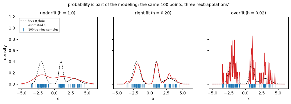
Four things to notice in this table:
- The training likelihood rises monotonically as shrinks and tends to as . The reason is simple: at a training point itself, . Judged only by “the likelihood of the training data”, the best model memorizes the training set.
- The held-out likelihood and the KL first improve, then get worse, with the best value at . A too-large smears the three peaks into one blob. A too-small leaves large “almost-zero-density” gaps between training points, and the log-likelihood of new data falling there collapses (−99 at ).
- An overfitted model copies when it generates. At , 97.1% of the generated samples are within 0.01 of a training point (only 37.2% of real new samples are). It can “generate”, but nothing new.
- Even “a rule for choosing the bandwidth” hides a modeling assumption. The textbook Silverman rule of thumb gives , several times larger than the best. The rule is derived assuming “the data look like one Gaussian”, and is wrong for three-peaked data.
One more noteworthy detail: the chosen by the held-out likelihood and the chosen by the KL are identical. We cannot compute the KL without the formula of , but we can compute the held-out likelihood — and §5 proves that the two differ only by a constant.
4.6 More data, more flexible models
Part 2 of script 04 varies the sample size , each time choosing the best bandwidth on a validation set:
| training samples | chosen on validation | Silverman’s | |
|---|---|---|---|
| 20 | 0.352 | 1.097 | 0.0791 |
| 100 | 0.209 | 0.786 | 0.0690 |
| 1,000 | 0.124 | 0.467 | 0.0118 |
| 5,000 | 0.124 | 0.341 | 0.0039 |
( and land on the same candidate bandwidth because there are only 16 candidates.) The more data, the more flexible the right model and the more accurate the learned distribution. “How flexible is right” is not decided by the model itself but by the amount of data — exactly the bias–variance trade-off of discriminative models. Deep generative models face the same problem, only “flexibility” is no longer a single knob but the architecture, the number of parameters, the training steps, regularization… Lecture 2’s Deep Image Prior gives a striking example: the network architecture itself is a strong prior.
5. Generative models with probabilistic modeling
5.1 The pipeline
The slides describe the pipeline of “generative models with probabilistic modeling” with a sequence of figures:
  data {x_1, ..., x_N}
        │  ← "the data follow some distribution": this step is itself modeling
        ▼
  the data distribution p_data
        │  ← optimize a loss (measuring the gap between two distributions)
        ▼
  the estimated distribution p_θ
        ├──→ sampling: generate new "data"
        └──→ probability density estimation: p_θ(x) = ? (optional)
The last step has two uses: sampling (generate new samples) and estimating probability densities (given an , how likely is it — for anomaly detection, compression, comparing models). Some models do both (autoregressive models, normalizing flows), some only sample (GANs), some only give a lower bound on the density (VAEs).
The slides add four “notes” here, worth taking one at a time:
- The statistical models in generative models are often designed and derived by humans. “Data = latents + rendering”, “each conditional is Gaussian”, “the noising process is like this” — all human choices.
- Probabilistic modeling is not only the neural network’s job. The network is responsible for only one part (§6.3).
- Probabilistic modeling is a popular approach, but not the only one. For example, a GAN’s generator never writes down explicitly, and Efros–Leung has no explicit probability model at all.
- “All models are wrong, but some are useful.” — the statistician George Box.
5.2 Measuring the gap between two distributions: KL divergence and maximum likelihood
The “loss” in the pipeline must measure how far apart and are. The classic choice is the KL divergence (Kullback–Leibler divergence):
It is always , and 0 only when the two distributions are equal everywhere (provable with Jensen’s inequality, exercise 5). But we do not know the formula of — how can we compute it? Split the log:
The first term is the negative entropy of the data distribution, a constant independent of the model. So:
Minimizing the KL divergence = maximizing the likelihood, and the latter needs only data samples and the model’s density, not the formula of . This is the one-line “tl;dr” at the start of the VAE lecture’s slides (original Lecture 2, Lecture 3 of these notes). Equivalently, the mean negative log-likelihood (NLL) satisfies
Part 1 of script 05 verifies this identity numerically. The true distribution is . For five different models, the NLL comes from 200,000 samples and the KL from numerical integration:
| model | NLL (sample mean) | KL (numerical integral) | NLL − KL |
|---|---|---|---|
| 3.6044 | 1.9106 | 1.6938 | |
| 2.3159 | 0.6216 | 1.6943 | |
| moment-matched Gaussian | 2.2557 | 0.5614 | 1.6942 |
| two-peak mixture, but weights 0.5/0.5 | 1.7125 | 0.0201 | 1.6924 |
| the true distribution | 1.6922 | 0.0000 | 1.6922 |
The last column equals the entropy of the data distribution for every model (differences come only from Monte Carlo error). Two consequences:
- ranking models by NLL is ranking them by KL;
- the floor of the NLL is the entropy of the data, not 0 — the data themselves are uncertain, and no model can remove that.
This also explains why “the held-out likelihood and the KL chose the same bandwidth” in §4.5.
5.3 The two directions of KL: blur or miss
The KL divergence is asymmetric: . The slides of the VAE lecture have a side note: “could we consider criteria other than KL?” Before answering it, look at what happens when the direction is switched.
- Forward KL : where but , blows up — wherever the data are, the model must be. It punishes “missing data” and does not much care if the model puts probability where there is no data. (Also called “mass-covering”.)
- Reverse KL : heavily punished where but — wherever the model is, the data must be. It punishes “inventing things” and does not much care about missing part of the data. (Also called “mode-seeking”.)
When the model family is large enough to contain the true distribution, both directions are optimized by , and there is no difference. The difference appears when the model family is too narrow. Part 2 of script 05 fits one Gaussian to two peaks:
| fit | samples between peaks | missed data | ||||
|---|---|---|---|---|---|---|
| forward KL (maximum likelihood) | −0.200 | 2.309 | 0.561 | 1.338 | 32.8% | 0.2% |
| reverse KL, starting at | −1.995 | 0.617 | 9.974 | 0.510 | 1.7% | 39.8% |
| reverse KL, starting at | +0.558 | 2.109 | 0.635 | 1.099 | 30.8% | 0.1% |
| reverse KL, starting at | +2.493 | 0.840 | 7.972 | 0.914 | 4.1% | 60.1% |
(“Samples between peaks”: the fraction of model samples where the true density is < 0.02; “missed data”: the fraction of real data where the model density is < 0.02.)
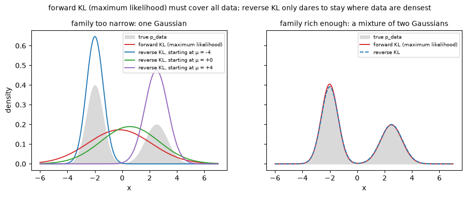
- The forward-KL solution is “moment matching”: the same mean and variance as the data, one wide Gaussian spanning both peaks. It misses almost no data, but about a third of its samples fall between the peaks — blur. This is the distribution-level version of the “ghosts” of §2: to cover every possibility it has to smear across the middle. Part of the reason why models trained by maximum likelihood (VAEs, autoregressive models) produce “blurry”, “average” samples lies here.
- Reverse KL, started from either side, shrinks onto the nearer peak: its samples are almost all “real” (only 2–4% fall between the peaks), but the other peak’s data are dropped entirely (40% or 60%) — miss. This is the seed of the “mode collapse” of the GAN lecture.
- A result these notes did not anticipate: started right in the middle at , reverse KL stops at a “wide, fat” solution (unchanged even after 10,000 steps). A scan over (best for each ) shows that reverse KL has three local optima here: two narrow solutions (KL 0.51, 0.91) and this wide one (KL 1.10). The landscape of reverse KL is bumpy, and the result depends on the initialization.
Part 3 of script 05 switches the family to “a mixture of two Gaussians” (which contains the truth). Both directions recover the true parameters: weights 0.61/0.39 and 0.60/0.40, with KL below 0.001 in both cases.
5.4 “All models are wrong”
These experiments make George Box’s remark concrete. In real problems the model family never contains exactly, so the choice of objective decides which kind of error the model makes — blur (forward KL / maximum likelihood) or miss (reverse KL).
There is also a practical difference. Forward KL needs only data samples. Reverse KL must evaluate on the model’s samples — and in reality there is no such formula. Later families answer this in different ways:
- GANs (Lecture 9) get around it with a discriminator, and can be shown to optimize a different divergence (the JS divergence);
- diffusion models and flow matching (Lectures 12, 16) give a third kind of answer: they turn learning a distribution into a sequence of regression problems.
6. Deep generative models
6.1 Deep learning is representation learning
The slides place deep learning in one sentence: deep learning is representation learning. It has two kinds of “representation”:
- Learning to represent data instances: map data to features , then train with a goal-directed loss, e.g. the classification loss . This is what discriminative deep learning does: ResNet represents an image as features, followed by a classifier.
- Learning to represent probability distributions: map a simple distribution (Gaussian / uniform) to a complex one, , , so that the distribution pushed forward by is close to the data distribution. The loss is some gap to the data distribution, . This is what generative deep learning does.
And the two are often done together. A VAE’s encoder “represents data instances” (compresses an image into a latent vector) while its decoder represents the distribution. The tokenizers of today’s text-to-image models (Lectures 3, 7, 9) first represent images as compact latents, and the generative model then represents the distribution in that latent space.
The second kind of representation is exactly what §4 described: “simple latents + a nonlinear map = a complex distribution”. In GlyphWorld the map is the renderer we wrote. What a deep generative model must do is learn such a map from data with a neural network — or learn something equivalent: a sequence of conditionals, a denoiser, a velocity field, …
6.2 Not every part is learned
The slides then stress an easily overlooked fact: many parts of distribution modeling are not learned but designed. Two cases:
- Autoregressive models: writing as — this dependency graph (who depends on whom, in which order) is designed by people; the mapping of each conditional is learned (e.g. by a Transformer).
- Diffusion models: the “noising” process from data to noise and the dependency graph of the “denoising” direction are designed by people; the mapping of each denoising step is learned (e.g. by a U-Net).
This is why the “formulation” mentioned in §0.5 matters: the same network architecture combined with different dependency graphs / noising processes gives entirely different models. Script 06 shows the weight of “design” with a concrete example.
6.3 Five components
Putting the discussion together, the slides list five parts a deep generative model may contain:
| component | question it answers | examples |
|---|---|---|
| formulation | How is the problem written as probabilistic modeling? How is a complex distribution factorized into simple, tractable ones? | the chain rule (autoregressive); latents (VAE); a sequence of noising / denoising steps (diffusion) |
| representation | Which deep networks represent the data and their distributions? | MLP, CNN, Transformer, U-Net; outputting a categorical distribution / Gaussian parameters / noise / velocity |
| objective | How do we measure how good the predicted distribution is? | likelihood / KL, ELBO, adversarial loss, score matching, flow matching |
| optimization | How do we optimize the networks (and the factorization)? | stochastic gradient descent, minimax, the alternating optimization of EM |
| inference | How do we use the learned model? | a sampler (produces new samples); a probability density estimator (optional) |
Every model in the course can be dissected with this table. Take a GAN:
- formulation = noise mapped to samples by a generator;
- representation = two networks, a generator and a discriminator;
- objective = the adversarial loss;
- optimization = alternating gradient steps of a minimax game;
- inference = sampling with one forward pass, with no density estimate.
6.4 Experiment: a deep generative model that is “small but complete”
Script 06 builds the smallest autoregressive model on a 2-D distribution: uniform, along a sine curve with a little noise. It maps the five parts onto code one by one:
- Formulation: cut into 32×32 cells (discretization) and use the chain rule .
- Representation: as 32 learnable numbers (logits); as a small MLP (input the cell index of , output logits over the 32 cells of ).
- Objective: the negative log-likelihood — the sum of the cross-entropies of two “classification” problems.
- Optimization: Adam, minibatches, 2000 steps.
- Inference: sampling = draw , then (“ancestral sampling”); density = compute directly.
Then five variants, with the same data and the same training:
| model | bits per dimension (bits/dim) | gap (KL per dim) | TV distance of the sample histogram |
|---|---|---|---|
| A: , categorical | 3.7192 | 0.0145 | 0.072 |
| B: , categorical | 3.7246 | 0.0198 | 0.085 |
| C: , unimodal Gaussian | 3.7171 | 0.0124 | 0.061 |
| D: , unimodal Gaussian | 4.4531 | 0.7483 | 0.586 |
| E: , independent | 4.7173 | 1.0125 | 0.715 |
(Floor: the entropy of the discretized true distribution = 3.7048 bits/dim; two independent uniforms = 5 bits/dim.)
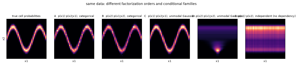
- A and B are both close to the entropy floor: the chain rule holds for any order, and with flexible categorical conditionals both orders learn well.
- C (unimodal Gaussian, first) is also very good, even slightly better than A. Given , is a small blob near the sine curve, which one Gaussian fits exactly; and with only 2 numbers per conditional it overfits less than 32 logits.
- D (unimodal Gaussian, first) clearly fails. Given , can be at two or three places on the sine wave (multimodal), and one Gaussian can only smear them together (the forward KL of §5.3). Same data, same network, only the factorization order changed. The autoregressive lecture’s slides (original Lecture 3, Lecture 5 of these notes) put it this way: “both factorizations are correct, but one may be much easier to learn than the other”. The dependency graph is designed, and its quality decides success or failure.
- E (no dependency): both marginals are right, but their relationship is lost; samples form a big block instead of a wave — just like “independent pixels” in §4.3.
Finally, the same model both samples and gives the exact probability of any cell. Model A gives 0.00886 for a cell on the band (true value 0.00858), and for a cell far from the band (true value 0). An autoregressive model’s “inference” has both.
Why “bits per dimension”? The negative log-likelihood in base 2, divided by the dimension, is “how many bits on average to encode one dimension”. It ties directly to compression: a good probability model is a good compressor. The “bits/dim” common in image-generation papers is this quantity.
7. Formulating real-world problems as
7.1 The roles of and
The last part of the slides unifies all these applications in one sentence: a generative model is .
| can be | can be |
|---|---|
| condition | “data” |
| constraint | samples |
| labels | observations |
| attributes | measurements |
| more abstract | more concrete |
| less information | more information |
7.2 Cases
The slides list these cases one by one (grouped slightly here):
| task | ||
|---|---|---|
| natural-language dialogue | a prompt | the chatbot’s reply |
| text-to-image / text-to-video | a text prompt | the generated visual content |
| text-to-3D | a text prompt | the generated 3-D structure (the slides’ example: LGM, ECCV 2024) |
| protein structure generation | conditions / constraints (e.g. symmetry) | the generated protein structure (RFdiffusion) |
| class-conditional image generation | a class label (e.g. “red fox”) | the generated image (the slides’ example was generated by MAR) |
| “unconditional” image generation | an implicit condition: “images like CIFAR-10” | generated CIFAR-10-like images (EDM) |
| classification (generative view) | an image (as the “condition”) | class probabilities conditioned on the image |
| open-vocabulary recognition | an image | plausible descriptions (“bird”, “flamingo”, “red”, “orange”, …) |
| captioning | an image | a plausible text description |
| chat with visual input | an image + a text prompt | the chatbot’s reply (an example from the GPT-4 technical report) |
| robot policy learning | visual and other sensor observations | the policy (probabilities of actions; Diffusion Policy) |
A few points worth pausing on:
- “Unconditional” generation has a condition. is the distribution of “all images”; an “unconditional” model trained on CIFAR-10 learns . The condition hides in the choice of dataset.
- Classification is also , with the roles swapped: the image is the condition , the class the to generate. From this angle a discriminative model is a special case of a generative one — with a tiny output space and an almost deterministic conditional.
- Open-vocabulary recognition shows that even “recognition” can have non-unique answers: for a photo of a flamingo, “bird”, “flamingo”, “pink” and “standing in water” are all plausible descriptions. Once the output space becomes open and complex, recognition becomes a generative problem too.
- Robot policies: under the same observation the robot may go around the left or the right; demonstration data are multimodal. Writing the policy as and representing it with a generative model (Lecture 21) avoids the “averaging” of §2 that would steer the robot into the obstacle.
The slides close with three questions: What is ? What is ? How do we represent , and the dependency between them?
7.3 Experiment: the more abstract , the more “generative” the problem
” is more abstract, with less information” can be measured precisely with information theory. The conditional entropy measures “how much uncertainty about remains once is given” (in bits; can be roughly read as “the average number of equally plausible answers”):
Script 07 builds a small glyph world where every possibility can be enumerated: 10 digits × 3 dx × 3 dy × 2 thicknesses × 3 slants = 540 equally likely combinations, rendering 540 distinct images, so bits. For the same (the image), seven different :
| condition | corresponding task | mutual information | most answers | ||
|---|---|---|---|---|---|
| ∅ | unconditional generation | 9.077 | 540.0 | 0.000 | 540 |
| even or odd | attribute-conditional generation | 8.077 | 270.0 | 1.000 | 270 |
| digit class | class-conditional generation (“draw a 7”) | 5.755 | 54.0 | 3.322 | 54 |
| digit + position | generation with a layout constraint | 2.585 | 6.0 | 6.492 | 6 |
| 4×4 three-level thumbnail | super-resolution | 1.457 | 2.7 | 7.619 | 26 |
| top half of the image | image completion | 0.584 | 1.5 | 8.493 | 3 |
| all latents | rendering (deterministic map) | 0.000 | 1.0 | 9.077 | 1 |
As goes from “nothing” to “all latents”, falls from 9.08 all the way to 0. The more abstract and the less information it carries, the more possibilities has and the more “generative” the problem; when determines completely, the problem degenerates into a function — and regression is enough (the unambiguous inputs of §2.4). The two “image conditions”, super-resolution and completion, carry a lot of information but still leave a little ambiguity (1.5–2.7 candidates on average, at most 26) — exactly why they need generative models.
Now classification ( = the digit label, = the image):
| condition | most candidate labels | |
|---|---|---|
| full image | 0.000 | 1 |
| 4×4 three-level thumbnail | 0.466 | 7 |
| top half of the image | 0.584 | 3 |
| nothing | 3.322 | 10 |
Given the full image the label’s entropy is 0: classification is a whose “output is almost certain”. Given only the top half, about 0.6 bit remains:
- with the digit centered, it is a choice between two: 2/3, 5/6 or 8/9;
- with the digit shifted down, even the middle bar g is invisible, and it is a choice among three: 0/8/9 or 2/3/7;
- with the digit shifted up, a piece of the bottom half shows, and there is no ambiguity.
A final observation: . “Generating an image from a label” is hard precisely because the extra ~5.8 bits must be filled in — what the slides mean by “the output is more complex and more informative than the input”. In real text-to-image, a sentence may carry only tens to hundreds of bits, while an image carries far more.
Script 07 ends by enumerating / sampling directly from several conditional distributions, so you can see that “several under the same all satisfy the condition and yet differ from each other” — exactly what must represent. Real problems cannot be enumerated (images have thousands of dimensions, styles are continuous), so a neural network must represent the conditional distribution, and we must be able to sample from it.
8. The big picture
8.1 Three things this course covers
The last slide: this course covers
- how real-world problems are formulated as generative models (§7 of this lecture; the applications of Lectures 19–24);
- probabilistic foundations and learning algorithms (the model families of Lectures 3–18);
- challenges, opportunities and open problems (throughout the reading sessions).
8.2 The model families at a glance
Later lectures develop every row of this table. For now, remember that they all answer the question of §6.3: “how do we factorize a complex distribution into simple ones?”
| family | how it represents a complex distribution | sampling | density? | training | typical problems | lectures |
|---|---|---|---|---|---|---|
| VAE | simple latents + a decoder | one forward pass | lower bound (ELBO) | stable (maximize the ELBO) | blurry samples | 3 |
| normalizing flows | a sequence of invertible maps | one forward pass | exact | stable (maximum likelihood) | restricted architecture, dimension cannot change | 4 |
| autoregressive | the chain rule, one element at a time | element by element, steps = sequence length | exact | stable (cross-entropy + teacher forcing) | slow sampling; needs an order / a tokenizer | 5–8 |
| GAN | generator + discriminator as the loss | one forward pass | no | minimax, unstable | mode collapse, hard to converge | 9–11 |
| diffusion / score matching | a sequence of noising / denoising steps | many iterations | lower bound / via an ODE | stable (regress the noise) | slow sampling | 12–15 |
| flow matching | a velocity field transporting noise to data | many ODE steps (fewer if paths are straight) | via an ODE | stable (regress the velocity) | sampling still needs several steps | 16–17 |
| consistency models | jump to the end of an ODE trajectory in one step | 1 to a few steps | no | distillation or direct training | — | 18 |
Yang Song’s guest lecture (Lecture 18) has a slide “a catalogue of one-step generative models” that is a subset of this table:
- VAEs: stable training and likelihoods, but low sample quality.
- GANs: high sample quality, but unstable training and no likelihood.
- Flows: exact likelihoods, but restricted architectures and middling sample quality.
- Consistency models: stable training and high sample quality, but no likelihood.
No family dominates across the board, which is why this course compares them side by side.
8.3 This lecture’s place in the course
 Lecture 1 (this one): generation = represent and sample p(x|y); five components
     │
     ├─ Lecture 2: how "priors of natural images" were modeled before deep learning
     ├─ Lecture 3: latents (VAE / EM / VQ-VAE) -- the "latents + world model" of §4, learned by networks
     ├─ Lecture 4: invertible maps (flows) -- the "simple → complex distribution" of §6, with an invertible map
     ├─ Lectures 5-8: the chain rule (autoregressive) -- §6.4 scaled up; tokenizers; combining with diffusion
     ├─ Lectures 9-11: adversarial -- no KL, a network as the loss (the other path of §5.3)
     └─ Lectures 12-18: diffusion and flows -- "simple → complex" split into many small steps
9. Summary
- The hallmark of a generative problem is one-to-many: one input has a distribution of plausible answers. Regression (squared error) gives the mean of that distribution, which looks like nothing when there are several peaks (“ghosts”); a generative model must represent the distribution and sample from it. Per-pixel error inherently favours the mean: a perfect sampler has exactly twice the squared error of a perfect regressor.
- Discriminative and generative models are linked by Bayes’ rule: generative model + prior → discriminative model; discriminative model + → generative model. Gradient ascent on a discriminative model’s input finds the extreme of a boundary, not a typical sample. The challenge is representing and predicting distributions.
- Probability is part of the modeling.
- Simple latents passed through a nonlinear “world model” produce a complex data distribution; fitting simple models directly in pixel space fails, and latent space is the “flat” coordinate system.
- We only have finite data, so the model must extrapolate; hence underfitting and overfitting. δ functions = memorizing the training set.
- The more data, the more flexible the model can be.
- Maximum likelihood = minimizing ; NLL = entropy + KL. With a too-small model family, forward KL makes the model “blur” (cover all data) and reverse KL makes it “miss” (mode collapse). All models are wrong; the objective decides which error they make.
- Deep generative model = representing a distribution with deep networks: map a simple distribution to a complex one. Five components: formulation, representation, objective, optimization, inference. Dependency graphs, noising processes and the like are often designed; only the map is learned, and the quality of the design can decide success or failure.
- Everything is : is more abstract with less information, more concrete with more. The larger the conditional entropy , the more “generative” the problem; at it degenerates into a function. Classification is a special case of .
10. Common pitfalls
- “Generative model = unsupervised learning.” No. Today’s most important generative models (text-to-image, chat) are conditional generation ; even “unconditional” generation has an implicit condition (§7.2). Whether a generative model is needed depends on whether the output is one-to-many, not on whether there are labels.
- “The best generation outputs the most probable sample.” No. §2 showed that “averaging” fails; “the most probable point” (the mode) fails too. It has no diversity, and in high dimensions the most probable point is often highly atypical: the mode of a high-dimensional standard Gaussian is the origin, while almost all samples are about away. Generation needs sampling.
- “Lower squared error / higher PSNR is better, so generative models should compete on these.” For generative problems these metrics systematically favour “blurry” answers (§2.5).
- “The higher the training likelihood, the better the model.” The training likelihood can be pushed to infinity by memorizing the training set (§4.5). Look at the held-out likelihood, or at sample-level evaluations.
- “A discriminative model’s already contains the distribution of the data.” It does not. is “insensitive” to : however changes, as long as the class proportions at each stay the same, does not change. So a discriminative model cannot be used directly to generate (§3.5).
- “The KL divergence is a distance between two distributions.” It is asymmetric () and violates the triangle inequality, so it is not a distance in the mathematical sense; its two directions have completely different personalities (§5.3).
- “Everything in a deep generative model is learned.” Dependency graphs, factorization orders, noising processes, discretizations, tokenizers… many key choices are designed by people (§6.2, §6.4).
- “Autoregressive models are RNNs / only for time series.” Autoregression is a formulation (the chain rule), independent of the network architecture and not requiring a temporal order; the order and the partition can be chosen freely (Lecture 5).
- “The average of two images in pixel space should also be a plausible image.” The set of plausible images is not convex in pixel space (the interpolation experiment of §4.3). Interpolation is meaningful in latent space — provided the latent space is learned well.
11. Exercises
Exercise 1 (squared error and the conditional expectation) (a) Prove the decomposition of §2.3, and deduce that . (b) Prove: if and are i.i.d. given , then . (c) If the squared error is replaced by the mean absolute error (1-D), what is the optimal ? For the problem of §2.2, does it still give “impossible answers”?
Answer
(a) Let . . Take the expectation of the cross term given first: is a function of and can be pulled out, while , so the cross term has expectation 0. Hence , with equality iff (almost everywhere).
(b) Given , . By independence the last expectation factors into an inner product of two expectations, each 0; the first two terms are equal (same distribution). Then take the expectation over .
(c) The optimum of the mean absolute error is the conditional median. For , puts 1/2 on each of , so any number in is a median — including 0. So switching to the absolute error does not solve the problem: no objective that “outputs one point” can express “both are fine” in the face of two symmetric peaks. The problem is “outputting one point” itself, not the particular error used.
Exercise 2 (the posterior of a generative classifier is a logistic function) A 1-D two-class problem: (equal variances), prior . Show and give , . How does the result change if the variances differ? How does this relate to why script 02 gives logistic regression quadratic features?
Answer
. So , , and .
With different variances the terms no longer cancel, and the log-odds are a quadratic function of (a quadratic form in several dimensions). In script 02 the two classes have different covariances, so the generative classifier’s (QDA’s) decision boundary is a quadratic curve. Only with quadratic features does logistic regression’s boundary belong to the same family, which makes the comparison fair.
The exercise also shows that the assumptions of a generative model decide the form of the discriminative model it induces.
Exercise 3 (correcting for a changed prior) During training the class prior is ; at test time it becomes , while the within-class distributions do not change. Show that the test-time posterior is . Why do we say the correction “quietly uses the generative view”?
Answer
and . Substituting, ( is a constant for a given ). The key step of the derivation is ” does not change” — an assumption about how data are produced from classes, i.e. a generative assumption. A purely discriminative model does not itself know that “the prior changed but the within-class distributions did not”.
Exercise 4 (δ functions and the training likelihood) For the kernel density estimate of §4.5, show that the mean training log-likelihood as (with distinct training points). And for a new point not in the training set,
Answer
. So . For a new point at distance from the nearest training point, , so ( grows much faster than ). This is why the held-out likelihood collapses to −99 at in the table.
Exercise 5 (non-negativity of KL) Use Jensen’s inequality ( is concave, so ) to prove . When does equality hold? Deduce that “the floor of the NLL is ”.
Answer
. Equality holds iff is almost everywhere constant on the support of , which together with both integrating to 1 means (almost everywhere). From the floor follows, attained only when .
Exercise 6 (the forward-KL-optimal Gaussian is moment matching) Let and any 1-D distribution with mean and variance . Show that is attained at , . For , write the optimal , and compare with the result of script 05 (where ).
Answer
. Since , minimizing over gives . Substituting back and differentiating in : , so .
For the symmetric two peaks, and , so the optimal — spanning both peaks exactly.
Script 05: ; , so . This matches the table’s , .
Exercise 7 (the parameter count of the chain rule) How many free parameters does a full probability table for the joint distribution of binary variables need? What about an autoregressive factorization with every conditional also stored as a full table? And with every conditional a logistic regression ? (This is the problem the Bengio & Bengio 1999 paper of Lecture 6 sets out to solve.)
Answer
- Full joint table: (the probabilities of all combinations, minus the “sums to 1” constraint).
- Autoregressive + full conditional tables: the -th conditional needs one number per value of , for a total of . The chain rule itself involves no approximation, so the count is the same as the full table.
- Logistic-regression conditionals: the -th has weights plus 1 bias, for a total of . That is down from exponential to quadratic, at the price of assuming the form of the conditionals (the “approximation brought by inductive biases” of §6.2).
Neural networks with shared weights can strike a better balance between the two.
Exercise 8 (writing tasks as ) For each task below, give and , say which carries more information, and whether is roughly “large”, “medium” or “close to 0”: (a) machine translation; (b) weather forecasting (given the last hour of radar maps, predict the next hour); (c) speech recognition; (d) text-to-speech; (e) colorizing black-and-white photos.
Answer
(a) = the source sentence, = the target sentence. Similar amounts of information, but one meaning has several plausible translations: medium.
(b) = past radar maps, = future radar maps. carries more information (the details of the future cannot be fully determined by the past), and grows with the forecast horizon. This is exactly why Ravuri et al. 2021 used a generative model rather than regression: regression forecasts get blurrier with time.
(c) = speech, = text. Speech carries much more information; is close to 0 (apart from a little ambiguity such as homophones) — close to a discriminative problem.
(d) = text, = speech. The same sentence can be read with countless voices, intonations and rhythms; is large — a typical generative problem. Note that (c) and (d) are the two directions of the same pair .
(e) = a grayscale image, = a color image. A piece of clothing can be red or blue: medium. Colorizing with L2 regression gives “grayish, brownish” average colors — the color version of the ghosts of §2.
Exercise 9 (hands-on)
(a) In 01_one_to_many.py, change the number of neighbours to 1 and to 50. How do the “crisp” fractions of the nearest-neighbour average and nearest-neighbour sampling change? Explain why.
(b) In 06_tiny_deep_generative_model.py, change GaussianConditional to a mixture of three Gaussians (the network outputs 3 sets of , and 3 mixture weights). How low can model D’s bits/dim go? What does this say about the role of the “representation” component?
Answer (sketch)
(a) With , the nearest-neighbour average equals nearest-neighbour sampling (there is only one neighbour); both become “copy the nearest image”, with a crisp fraction close to nearest-neighbour sampling. With , the two digits each make up about half of the 50 neighbours, so the nearest-neighbour average is almost all ghosts (crisp fraction near 0). Nearest-neighbour sampling’s crisp fraction drops slightly, because the neighbours’ styles differ more and the copied bottom halves line up worse. How much you average decides how “blurry” the result is.
(b) Given , falls at most at three places on the sine wave, and a mixture of three Gaussians is enough to represent this multimodal conditional. Model D should approach the level of A and B (exact numbers from your own run). This shows that a poorly chosen factorization order can be compensated by a more flexible representation (conditional family); conversely, a good factorization lets a simple representation suffice. “Formulation” and “representation” have to be designed together.
12. Further reading
Works cited on the slides of this lecture
- A. A. Efros & T. K. Leung, Texture Synthesis by Non-parametric Sampling, ICCV 1999. (§1.2; optional reading in Lecture 2)
- C. Barnes, E. Shechtman, A. Finkelstein, D. B. Goldman, PatchMatch: A Randomized Correspondence Algorithm for Structural Image Editing, SIGGRAPH 2009. (§1.3; optional reading in Lecture 2)
- W. T. Freeman & J. B. Tenenbaum, Learning Bilinear Models for Two-Factor Problems in Vision. (source of the figure in §4.1)
- J. L. Watson et al., De novo design of protein structure and function with RFdiffusion, Nature 2023. (§1.1, §7.2; required reading in Lecture 23)
- S. Ravuri et al., Skilful precipitation nowcasting using deep generative models of radar, Nature 2021. (§1.1)
- J. Tang et al., LGM: Large Multi-View Gaussian Model for High-Resolution 3D Content Creation, ECCV 2024. (§7.2)
- T. Li et al., Autoregressive Image Generation without Vector Quantization, 2024. (§7.2; required reading in Lecture 8)
- T. Karras et al., Elucidating the Design Space of Diffusion-Based Generative Models, NeurIPS 2022. (§7.2; optional reading in Lecture 13)
- C. Chi et al., Diffusion Policy: Visuomotor Policy Learning via Action Diffusion, RSS 2023. (§7.2; required reading in Lecture 21)
- OpenAI, GPT-4 Technical Report, 2023. (§7.2)
Textbooks and surveys
- K. P. Murphy, Probabilistic Machine Learning: Advanced Topics (2023), Part IV “Generation”: a systematic treatment of VAEs, autoregressive models, flows, GANs and diffusion, with unified notation.
- C. M. Bishop & H. Bishop, Deep Learning: Foundations and Concepts (2024): clear chapters on generative models with just the right amount of mathematics.
- I. Goodfellow, Y. Bengio, A. Courville, Deep Learning (2016), Chapter 20: the landscape of deep generative models before the GAN era.
- G. E. P. Box, Science and Statistics, JASA 1976: one source of the famous remark of §5.1.
Blogs (recommended by the original course as examples for final-project blogs)
- Yang Song, Generative Modeling by Estimating Gradients of the Data Distribution (2021).
- Sander Dieleman, Perspectives on diffusion (2023).
- Lilian Weng, Diffusion Models for Video Generation (2024), and her series on VAEs / GANs / flows.
Related notes in this repository (in Chinese)
- MIT6.S184 Lecture 1: building generative models with differential equations, starting from “generation is sampling”.
- CMU10-423: a panorama of generative AI, with introductory notes on VAEs, GANs and diffusion.
13. Next lecture
Lecture 2: Image priors — generative models before deep learning (original reading session · 09/10).
§1 of this lecture showed that the core ideas of generative models appeared as early as 1999. Lecture 2 goes back to the pre-deep-learning era and asks a more specific question: what makes an image “natural”? The three required papers give three answers:
- Zoran & Weiss (2011): a Gaussian mixture prior learned on 8×8 patches (EPLL) gives the best denoising and deblurring of its time — the “prior” is the core of image restoration;
- Zoran & Weiss (2012): why do Gaussian mixtures work so well for natural images? The answer hides in a simple generative process called the “dead leaves model”: occlusion and scale invariance;
- Ulyanov et al. (2018, Deep Image Prior): the architecture of a completely untrained convolutional network is itself a strong image prior.
We will implement EPLL denoising, the dead leaves model, Efros–Leung texture synthesis, PatchMatch, and a Deep Image Prior on a small CNN, using GlyphWorld and synthetic textures.