Maps to: MIT 6.S978 Deep Generative Models (Fall 2024), Lecture · Thu 09/12/2024 · Variational Autoencoder (VAE) (Kaiming He’s slides
lec2_vae.pdf), plus Problem Set 1 (autoencoders, the SGVB estimator and the analytic KL, a VAE on a torus point cloud; released 09/10, due 09/24). Basis: The skeleton follows the slides: latent-variable models → why the likelihood is hard → a tractable q → the ELBO → the VAE objective (reconstruction + regularization, the reparameterization trick) → the “autoencoding distributions” view → VAE vs EM vs K-means → VQ-VAE as a tokenizer. The slides state many steps in one line; this lecture fills in the derivations (the analytic KL, the EM monotonicity proof, the K-means limit, the ELBO decomposition) and adds the intuition for each design choice. All experiments were designed for these notes and run on a CPU in GlyphWorld (the seven-segment digit world of Lecture 1). Several outcomes contradicted my plan, and they are reported as they came out. Code:code/lecture03/— 6 scripts + the shared modulesglyph_kit.py(data and a “judge” for generated images, used from now on) andvae_tools.py. Each script runs in 3–60 s. Reading time: 4–5 hours including running the code.
0. How to read this lecture
0.1 Where we are
Lecture 1 said that probability comes from latent variables + a world model: GlyphWorld draws a few simple knobs (digit, shift, slant, thickness, …) and renders them deterministically into a complex 256-pixel image. Lecture 2 met the simplest learned latent-variable model, the Gaussian mixture over image patches: “first pick a component k, then generate linearly inside it”. It was trained with EM.
This lecture takes that idea to its conclusion:
- the latent becomes a continuous vector z;
- “generate linearly” becomes a neural-network decoder p_θ(x | z).
The decoder can represent almost anything, but we pay for it twice:
- The likelihood p_θ(x) = ∫ p(z) p_θ(x|z) dz becomes an integral nobody can compute.
- The posterior p_θ(z | x) — “which z produced this image?” — no longer has a formula.
The VAE (Kingma & Welling 2014; Rezende, Mohamed & Wierstra 2014) answers both problems with one trick:
- introduce a second distribution q(z | x) that we can handle;
- optimize a lower bound of the likelihood, the ELBO, instead of the likelihood itself.
The rest of the lecture looks at that trick from several angles:
- what the gap costs: §2–§3;
- how to compute its gradient: §4;
- what the latent space looks like: §5;
- how it relates to the older EM algorithm and to K-means: §6;
- how a discrete version, VQ-VAE, became the “tokenizer” of modern generative models: §7.
0.2 Learning goals
- Explain why the likelihood of a latent-variable model with a neural decoder is intractable, and what exactly is intractable: the integral and the posterior.
- Derive log p(x) = ELBO(q) + KL(q ‖ p(z|x)) from Bayes’ rule; explain why it holds for every q and what maximizing it over q and over θ each achieves.
- Write the VAE objective as “reconstruction − KL”; show that a Gaussian decoder gives an L2 loss and that σ plays the role of β; derive the closed-form KL between a diagonal Gaussian and N(0, I); explain the reparameterization trick and the two SGVB estimators.
- Distinguish the approximation gap from the amortization gap; explain why the reverse KL in the ELBO makes q “mode-seeking”; explain why training with the ELBO biases the model toward posteriors that are easy to approximate.
- Explain the aggregated posterior q(z), why it differs from the prior, what “holes” are, and what posterior collapse is.
- Show that EM is coordinate ascent on the same ELBO, prove that EM never decreases the likelihood, and derive K-means as the zero-variance limit of EM; explain why K-means is “an autoencoder and a (bad) generative model”.
- Explain VQ-VAE: the codebook, the codebook and commitment losses, the straight-through gradient, why there is no KL term, dead codes, and why a VQ-VAE still needs a separate model of the joint distribution of its tokens.
0.3 Map
| Section | Content | Code |
|---|---|---|
| §1 | Latent-variable models; why the likelihood is hard | — |
| §2 | The ELBO; the best Gaussian q; reverse KL | 01_elbo_gap.py parts 1–2 |
| §3 | Amortized inference; what ELBO training does to the model | 01_elbo_gap.py parts 3–4 |
| §4 | The VAE objective; Gaussian decoder; analytic KL; reparameterization; SGVB; β and posterior collapse; IWAE | 03_sgvb_and_kl.py |
| §5 | Autoencoding distributions: AE vs VAE, the aggregated posterior and holes; the torus | 02_ae_vs_vae.py, 06_torus_vae.py |
| §6 | VAE vs EM; K-means as EM and as an autoencoder | 04_em_and_kmeans.py |
| §7 | VQ-VAE: discrete latents, straight-through, codebooks, token priors | 05_vq_vae.py |
| §8 | The big picture: the five components, blurriness, where VAEs live today | — |
0.4 Notation
| Symbol | Meaning |
|---|---|
| x | data (a 16×16 image flattened to 256 numbers; in §5.4 a 3-D point) |
| z | latent variable; d = its dimension |
| p(z) | prior, here N(0, I) unless stated otherwise |
| p_θ(x | z) | decoder (likelihood); θ = its parameters |
| q_φ(z | x) | encoder / approximate posterior; φ = its parameters |
| ELBO(q) or L(θ, φ; x) | evidence lower bound |
| q(z) = E_{x ~ p_data} q_φ(z | x) | aggregated posterior |
| sg[·] | stop-gradient (.detach() in PyTorch) |
All log-likelihoods are in nats unless stated otherwise.
0.5 Problem Set 1 in this lecture
The original Pset 1 has four parts:
- an autoencoder;
- a VAE trained with the SGVB estimator (sampled KL);
- the same VAE with the analytic KL;
- a VAE on a point cloud sampled from a torus.
The derivations appear in §4 and the exercises (§11). The CPU versions of the coding parts are:
03_sgvb_and_kl.py(parts 1–2) for the two estimators;02_ae_vs_vae.pyfor the autoencoder comparison;06_torus_vae.pyfor the torus.
The original notebooks use MNIST and a GPU; doing them yourself is highly recommended after this lecture.
1. Latent-variable models · Why the likelihood is hard
1.1 A deep generative model maps a simple distribution to a complex one
The slides open with a picture you already know from Lecture 1: a simple distribution on z, a mapping g, and a complex distribution on x. In GlyphWorld the mapping is our renderer and z is 7 numbers. A deep generative model learns the mapping from data:
where f_θ is a neural network (the decoder). The model’s distribution over images is the mixture of infinitely many Gaussians, one for every z:
Why build a distribution this way instead of writing p(x) directly? Because “simple randomness pushed through a flexible function” is a very general way to make complicated distributions. It is also exactly how the world produces images: a few causes (identity, pose, lighting) pass through physics. The Gaussian mixture of Lecture 2 is the special case where z is a discrete index and f is a lookup of K mean vectors. The VAE replaces the lookup with a neural network and the index with a continuous vector.
1.2 The objective is still maximum likelihood
Lecture 1 §5.2 showed that minimizing KL(p_data ‖ p_θ) is the same as maximizing the expected log-likelihood E_{x ~ p_data} log p_θ(x). Nothing changes here: we want to maximize
1.3 What exactly is hard
Two things:
- The integral. For a neural decoder there is no closed form. We could estimate it by sampling z from the prior and averaging p_θ(x | z) (P1 §4). But almost every z from the prior generates an image that looks nothing like x, so p_θ(x | z) is astronomically small for nearly all samples and the estimate has enormous variance. The z’s that matter are concentrated in a tiny region.
- The posterior. That tiny region is the posterior p_θ(z | x) = p(z) p_θ(x|z) / p_θ(x). If we could sample from it, everything would be easy. But it needs p_θ(x) in the denominator, which is problem 1 again.
For the Gaussian mixture, both are easy: the integral is a sum over K components, and the posterior is the K “responsibilities”. This is why EM works for GMMs (§6). The neural decoder destroys both.
Intuition. Learning a latent-variable model is a chicken-and-egg problem. To improve the decoder we need to know which z explains each training image (the posterior). To know the posterior we need a good decoder. EM solves it by alternating exactly. The VAE solves it by learning a second network that guesses the posterior.
2. The ELBO · A lower bound we can optimize
2.1 Introduce a distribution we control
The slides’ move: pick any distribution q(z) that we can sample from and evaluate. Start from Bayes’ rule, which holds for every z:
Add and subtract log q(z), then take the expectation over z ~ q (the left side does not depend on z):
This identity holds for every q. Since the KL is non-negative, the first term is a lower bound on log p_θ(x): the Evidence Lower BOund (“evidence” is an old name for p(x)). P1 §4.3 checked this numerically for one toy model; here it is the backbone of the lecture.
Read it from both sides:
- With θ fixed, log p_θ(x) is a constant. So maximizing the ELBO over q is exactly minimizing KL(q ‖ true posterior) — the best q is the posterior itself, and then the bound is tight.
- With q fixed, the ELBO is a function of θ that never exceeds the log-likelihood. Maximizing it over θ pushes the likelihood up — as long as the gap stays small.
The ELBO contains no p_θ(x) and no p_θ(z | x), only the joint p_θ(x, z) = p(z) p_θ(x|z), which a neural decoder computes directly. That is the whole point.
2.2 Experiment: checking the identity exactly
01_elbo_gap.py builds a model small enough that everything can be computed by numerical integration over a fine grid:
The first coordinate is z², which cannot tell z from −z; the second coordinate θz carries a little sign information. So depending on x, the posterior can be unimodal or bimodal. Because log p(x|z) is a polynomial in z, the ELBO of a Gaussian q = N(m, v) has a closed form (Gaussian moments up to order 4). Meanwhile log p(x) and KL(q ‖ posterior) are integrated numerically, independently of the ELBO.
For x = (1.0, 0.2) and five very different q’s, all three quantities satisfy log p − ELBO − KL = 0 up to 3·10⁻¹¹:
| q(z) | log p(x) | ELBO(q) | KL(q ‖ posterior) |
|---|---|---|---|
| N(−1.0, 0.04) | −2.0067 | −4.7527 | 2.7460 |
| N(0.0, 1.00) | −2.0067 | −12.1522 | 10.1455 |
| N(0.9, 0.03) | −2.0067 | −2.1843 | 0.1776 |
| N(2.0, 0.50) | −2.0067 | −121.0543 | 119.0476 |
A bad q gives a loose bound, but never a wrong one.
2.3 The best Gaussian q, and why it only covers one mode
Now restrict q to Gaussians (as a VAE does) and find, for four values of x, the Gaussian with the largest ELBO. Equivalently, find the smallest KL(q ‖ posterior).
| case | P(z > 0 | x) | posterior mean / std | best q mean / std | gap of best q | gap of moment-matched q |
|---|---|---|---|---|---|
| A: unimodal (z ≈ 1.5) | 1.000 | +1.48 / 0.10 | +1.48 / 0.10 | 0.0034 | 0.0036 |
| B: bimodal, leaning right | 0.867 | +0.67 / 0.60 | +0.90 / 0.16 | 0.174 | 3.68 |
| C: bimodal, symmetric | 0.500 | 0.00 / 0.87 | −0.86 / 0.17 | 0.737 | 5.01 |
| D: near z ≈ 0 (unimodal, non-Gaussian) | 0.499 | 0.00 / 0.33 | 0.00 / 0.31 | 0.021 | 0.024 |

Two lessons:
- When the posterior is bimodal, the best Gaussian covers one mode and ignores the other. In the symmetric case C, the gap is 0.737 ≈ log 2: the q covers half of the posterior mass, and the bound pays roughly “one bit” (in nats, log 2) for not knowing the sign.
- The “obvious” Gaussian — the one with the right mean and variance — is far worse. Its gaps are 3.68 and 5.01 nat. The KL inside the ELBO is KL(q ‖ p), the reverse KL of Lecture 1 §5.3. It heavily punishes q for putting mass where the posterior is near zero. A wide Gaussian centered between the two modes puts most of its mass in the valley, which is the worst thing it can do. A narrow Gaussian sitting on one mode “misses” the other mode, but reverse KL forgives missing. This is the “mode-seeking” behaviour of reverse KL. Variational inference with a too-simple family almost always ends up here.
3. Amortized inference · And what the ELBO does to the model
3.1 From one q per x to an encoder
In §2.3 we optimized a separate q for each x. With 50,000 training images this would mean 50,000 small optimization problems at every training step, and another one for every new test image. The VAE’s second idea is amortization: train a single network, the encoder q_φ(z | x), that maps any x directly to the parameters of its q. The cost of inference is paid once, during training, and “amortized” over all future inputs.
This introduces a second source of error. The total gap splits into two parts:
This decomposition is due to Cremer, Li & Duvenaud (2018), “Inference Suboptimality in Variational Autoencoders”.
3.2 Experiment: where the two gaps live
Part 3 of 01_elbo_gap.py trains a 2 → 128 → 128 → 2 MLP encoder on 4000 points for 10,000 Adam steps. Because the ELBO here is analytic, the gradients have no sampling noise. On 2000 test points:
| test points | count | approximation gap (mean) | amortization gap (mean) | amortization gap (median) |
|---|---|---|---|---|
| all | 2000 | 0.076 | 0.777 | 0.003 |
| |x2| < 0.15 (bimodal) | 408 | 0.166 | 0.188 | 0.012 |
| x1 > 4 (|z| ≳ 2, rare) | 85 | 0.001 | 16.8 | 0.009 |
| the rest | 1507 | 0.056 | 0.032 | 0.002 |
What I expected was that the amortization gap would sit in the bimodal region. The reason: a smooth encoder cannot “switch modes” abruptly as x2 crosses 0. It is indeed larger there (0.188 vs 0.032), and 116 of the 140 test points where the encoder picks the wrong mode have |x2| < 0.15. But the mean is dominated by something else: rare inputs. When |z| ≳ 2 (x1 > 4), training data are scarce and the posterior is extremely narrow. Its std is about s/(2|z|), because z² changes fast there. A small extrapolation error by the encoder then costs a lot of ELBO. The worst 1% of test points account for 86% of the total amortization gap, while the median is only 0.003 nat. During development, a wider encoder and 3× longer training reduced the mean only slowly.
Takeaway. An encoder is a function approximator like any other: it is good where it has seen data and unreliable where it has not. Amortization error is not uniform; it hides in the tails.
3.3 Training θ with the ELBO biases the model
The ELBO is not only an approximation of the likelihood; it is a different objective, and maximizing it over θ prefers models whose posteriors are easy for the chosen q-family.
Part 4 of 01_elbo_gap.py shows this. Data come from θ* = 0.2: the sign information θz is weaker than above, so posteriors are often bimodal. For each θ on a grid of step 0.01, it computes:
- the exact mean log-likelihood;
- the mean ELBO when every x uses its own best Gaussian q (no amortization error at all).
| θ | mean log p(x) | mean best-Gaussian ELBO | mean gap |
|---|---|---|---|
| 0.15 | −1.7298 | −1.9542 | 0.224 |
| 0.20 (max likelihood) | −1.7223 | −1.9190 | 0.197 |
| 0.25 (max ELBO) | −1.7336 | −1.9088 | 0.175 |
| 0.30 | −1.7661 | −1.9238 | 0.158 |
The likelihood is maximized at the true θ = 0.20, but the ELBO at θ = 0.25. A larger θ makes x2 = θz more informative about the sign of z, so the posterior is more unimodal, more Gaussian, and the gap is smaller. The ELBO “buys” a smaller gap (0.197 → 0.175) with a slightly worse likelihood (−0.011 nat).
Honest note: with θ* = 0.5 the same effect exists but is tiny (the argmax moves by about 0.01). It only becomes visible when posteriors are often multimodal. In real VAEs the effect is real and well documented (Turner & Sahani 2011; Cremer et al. 2018). A VAE learns a decoder whose posterior its encoder can approximate. This is one reason VAE samples look “simpler” than the data.
4. The VAE objective
4.1 Rewriting the ELBO as reconstruction − regularization
Expand the joint p_θ(x, z) = p(z) p_θ(x | z) inside the ELBO, using q = q_φ(z | x):
The names come from reading this as an autoencoder:
- Reconstruction. Encode x into a cloud of codes q_φ(z | x), decode a sample, and score how well the decoded image matches x.
- Regularization. Keep each code cloud close to the prior N(0, I).
Without the second term this is an ordinary (noisy) autoencoder; §5 explains why the second term is what turns it into a generative model.
4.2 Gaussian decoder ⇒ L2 loss, and σ ⇔ β
With p_θ(x | z) = N(x; f_θ(z), σ² I) on d pixels:
So the reconstruction term is the squared error divided by 2σ² plus a constant. This is the slides’ “Gaussian decoder ⇒ L2 loss”. It also reveals a hidden hyperparameter. If σ is fixed (as in most implementations and in our code), multiplying σ by c multiplies the reconstruction weight by 1/c². That is equivalent to multiplying the KL weight by c². In other words, σ plays the role of β in the β-VAE (Higgins et al. 2017):
“Use MSE plus a KL term with some weight” and “use a Gaussian decoder with some σ” are the same model. §4.6 shows what the choice does.
4.3 Gaussian encoder + standard Gaussian prior ⇒ closed-form KL
Let the encoder output a mean μ(x) ∈ ℝ^d and a log-variance log σ²(x) ∈ ℝ^d, so q_φ(z | x) = N(μ, diag σ²). For one dimension:
using E_q[(z−μ)²] = σ² and E_q[z²] = μ² + σ². The dimensions are independent, so the KL is a sum over dimensions. Each term is ≥ 0 and equals 0 only when μ = 0 and σ = 1: a dimension with zero KL carries no information about x. The encoder outputs log σ² rather than σ because it is unconstrained, so any real number is valid.
4.4 The reparameterization trick
To train by gradient ascent we need ∇φ of E{q_φ(z|x)}[log p_θ(x | z)]. The expectation is over a distribution that depends on φ, so we cannot just move the gradient inside (P1 §5). The trick writes the sample as a deterministic function of φ and parameter-free noise:
Now the gradient flows from the decoder through z into the encoder like any other layer. P1 §5 compared it with the score-function (REINFORCE) estimator and found it far lower in variance for smooth f. A VAE uses a single sample of ε per training image: the noise averages out over the minibatch and over steps.
4.5 Two SGVB estimators: experiment
Kingma & Welling call the resulting Monte Carlo estimators “Stochastic Gradient Variational Bayes” (SGVB):
- Estimator A samples everything: log p(x|z) + log p(z) − log q(z|x) at one z.
- Estimator B samples only the reconstruction term and uses the formula of §4.3 for the KL.
Problem Set 1 implements both. 03_sgvb_and_kl.py, part 1, uses a trained 8-D VAE (σ = 0.1) and 500 test images:
| KL estimator | mean (nat) | std on one image |
|---|---|---|
| formula | 21.118 | 0 |
| 1 sample | 21.029 | 2.000 |
| mean of 1000 samples | 21.115 | 0.063 |
They are the same quantity; the one-sample version is noisy. Does that noise matter for training? Part 2 fixes 128 images and recomputes the gradient 200 times with fresh ε:
| estimator | parameters | total gradient variance | SNR ‖E g‖² / ΣVar |
|---|---|---|---|
| A | encoder | 2.473 × 10³ | 0.51 |
| B | encoder | 2.459 × 10³ | 0.51 |
| A or B | decoder | 3.347 × 10² | 1.88 |
The analytic KL reduces the encoder’s gradient variance by only 0.6%, and the two trained models reach the same test ELBO (318.05 vs 318.55). The textbook statement “B has lower variance” is true, but here the difference is negligible. The reason is visible in the formula:
- log q(z|x) − log p(z) depends on ε only through log p(z) = −‖μ + σε‖²/2;
- its gradient with respect to μ is −(μ + σε), with noise of size σε;
- this encoder’s posterior stds are small (median 0.066 on the active dimensions).
So the KL noise is tiny compared with the reconstruction term’s noise, whose std is 2.94 nat per image. Estimator B pays off when posteriors are wide.
4.6 σ (= β): rate, distortion and posterior collapse
Information theory gives the two ELBO terms names (Alemi et al. 2018):
- the KL term is the rate: how many nats the code carries about x;
- the reconstruction error is the distortion.
Trading one for the other traces a rate–distortion curve. Part 3 of 03_sgvb_and_kl.py trains 16-D VAEs with seven values of σ:
| σ | equiv. β | rate (KL, nat) | distortion (RMSE) | active dims / 16 | valid | mini FID |
|---|---|---|---|---|---|---|
| 0.03 | 0.09 | 53.7 | 0.025 | 16 | 0.305 | 780 |
| 0.05 | 0.25 | 39.6 | 0.025 | 16 | 0.397 | 357 |
| 0.1 | 1 | 22.4 | 0.028 | 10 | 0.578 | 64 |
| 0.2 | 4 | 14.6 | 0.034 | 8 | 0.715 | 56 |
| 0.4 | 16 | 9.2 | 0.048 | 7 | 0.745 | 41 |
| 0.8 | 64 | 2.7 | 0.145 | 3 | 0.443 | 481 |
| 1.6 | 256 | 0.0 | 0.228 | 0 | 0.000 | 1903 |
(An “active” dimension is one whose encoder mean varies across the data, Var_x μ_j(x) > 0.01; Burda et al. 2016. “Valid” and “mini FID” come from the judge of glyph_kit.py; see the code README.)
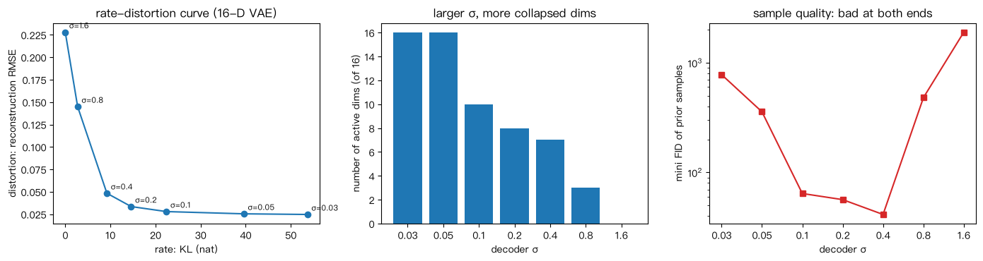
Three things happen as σ grows:
- Rate falls and distortion rises, as the trade-off says.
- Dimensions switch off one by one. A dimension’s KL drops to exactly 0, its posterior equals the prior, and the decoder ignores it. GlyphWorld has 7 underlying factors (the digit plus 6 styles); around σ = 0.1–0.4 the VAE uses 7–10 dimensions. At σ = 1.6 every dimension collapses: the reconstruction weight is so small that the best ELBO is reached by ignoring z altogether and outputting the mean image. This is posterior collapse. It also happens, for a different reason, when the decoder is so powerful (e.g. autoregressive) that it can model x without z (Bowman et al. 2016; Chen et al. 2017).
- Sample quality is worst at both ends. The best samples come at σ ≈ 0.4, not where reconstruction is best:
- with small σ the codes are very informative but spread out in a pattern the prior does not match (§5), so prior samples land in “holes”;
- with large σ everything is blurry or collapsed.
In practice the VAE inside Stable Diffusion uses a tiny KL weight, because there the decoder only needs to reconstruct; the generative modeling is done by a diffusion model in the latent space (§8).
The FID itself is noisy: four different sets of 2000 samples from the same σ = 0.1 model gave 57.1, 65.8, 59.8 and 58.6. Differences of a few points mean nothing.
4.7 How big is the gap in a real VAE? IWAE
In a real VAE we cannot integrate exactly, but the importance-weighted bound (IWAE, Burda et al. 2016; P1 §4.3) gives tighter and tighter lower bounds as the number K of samples grows:
For the 8-D VAE of §4.5 (200 test images), the bound rises above the ELBO (K = 1) by:
- +1.41 nat at K = 10;
- +1.93 nat at K = 100;
- +2.28 nat at K = 1000.
The true gap KL(q ‖ posterior) is at least 2.3 nat per image — small compared with an ELBO of about 320, but definitely not zero. IWAE can also be used as a training objective (Burda et al.), which tightens the bound at the cost of K decoder passes per image.
5. Autoencoding distributions · AE vs VAE, holes and topology
5.1 The slides’ view: distributions in, distributions out
The slides recast the VAE as an autoencoder of distributions:
- the encoder maps the data distribution p_data(x) to a distribution over codes, the aggregated posterior q(z) = E_{x ~ p_data} q_φ(z | x);
- the decoder maps code distributions back to image distributions.
Generation then works if — and only if — the distribution we sample from at test time (the prior p(z)) matches the distribution the decoder was trained on (q(z)).
What does the KL term do to q(z)? It acts on each q_φ(z | x) separately, not on q(z) directly. Averaging the KL over the data gives an exact decomposition (Hoffman & Johnson 2016, “ELBO surgery”; exercise 7):
The KL penalty has two jobs:
- it pushes the aggregated posterior toward the prior, which is what generation needs;
- it penalizes the information the code carries about x, which reconstruction needs.
The VAE cannot do the first without paying for the second. InfoVAE (Zhao et al. 2019) and adversarial autoencoders (Makhzani et al. 2016) drop the second part and match q(z) to p(z) directly.
5.2 Experiment: what an AE and a VAE do with their latent space
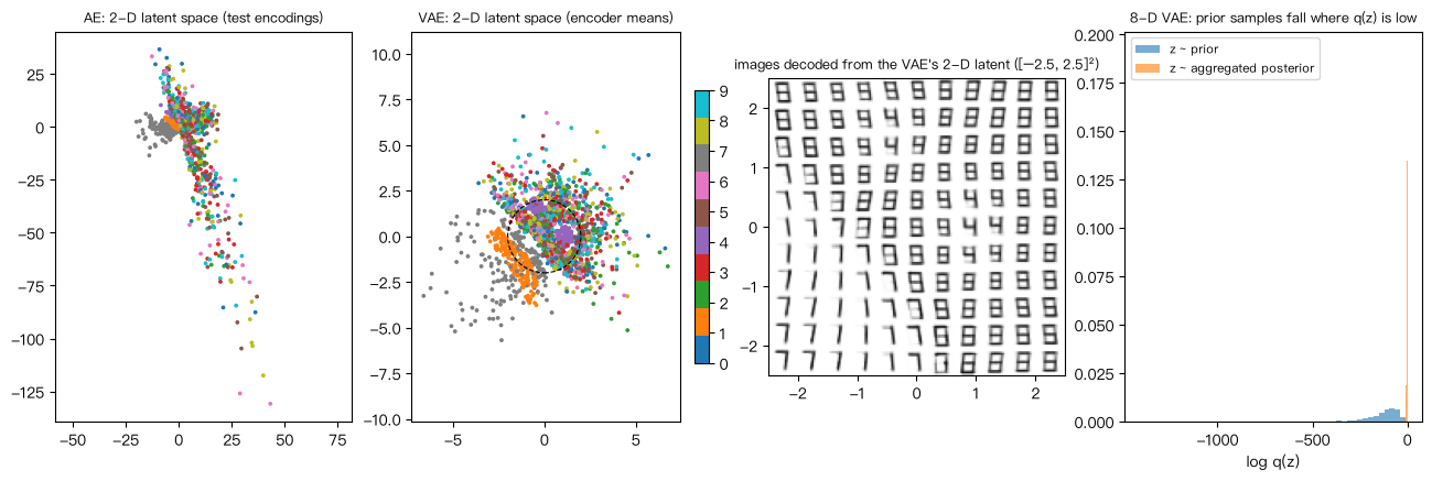
02_ae_vs_vae.py trains an autoencoder (encoder means only, no KL) and a VAE with the same networks and the same reconstruction weight (σ = 0.1).
2-D latents. The two models differ sharply in scale:
| model | latent mean | latent std | max |z| |
|---|---|---|---|
| AE | (+3.09, −1.97) | (6.55, 14.70) | 130.8 |
| VAE (encoder mean) | (+0.26, +0.15) | (1.68, 1.63) | 6.8 |
The AE’s latent scale is an arbitrary by-product of training; nothing tells it where codes should live. The VAE’s latents sit at the scale of N(0, I). The VAE encoder’s own std is tiny (median 0.027): with a heavy reconstruction weight, each code cloud is a narrow blob.
What does a 2-D latent encode? I expected the classic MNIST picture: ten digit clusters. It did not appear. A regression of each true style factor on the 2-D latent gives:
| model | digit η² | dx R² | dy R² | scale R² | slant R² | thick R² | ink R² |
|---|---|---|---|---|---|---|---|
| AE | 0.07 | 0.18 | 0.20 | 0.04 | 0.01 | 0.00 | 0.00 |
| VAE | 0.29 | 0.73 | 0.15 | 0.01 | 0.02 | 0.00 | 0.00 |
The VAE’s 2-D latent mostly encodes horizontal translation; “which digit” explains only 29% of its variance. The reason is the objective. The ELBO measures pixel error, and shifting a seven-segment glyph by one pixel changes more pixels than switching it to a different digit. So with only two numbers to spend, the model spends them on translation. A generative model’s latent space organizes the data by what its loss cares about, not by what we care about.
Prior samples (2-D):
| recognizable | class entropy (bit) | mini FID | |
|---|---|---|---|
| AE: z ~ N(0, I) | 0.904 | 1.58 | 1722 |
| VAE: z ~ N(0, I) | 0.622 | 2.16 | 340 |
The AE’s prior samples all fall in the small patch near the origin, which happens to decode to a few digit types (class entropy 1.58 of a possible 3.32). The VAE’s samples cover more digits, but 2 dimensions are too crowded: the transitions between digits decode into blurry hybrids.
5.3 8-D latents: is the VAE’s advantage just “the right scale”?
With 8 dimensions both models reconstruct well (RMSE 0.028 vs 0.029). The interesting comparison is a third generator: “AE + a Gaussian fitted to its latents after training”. It fixes the AE’s scale problem without a KL term.
| generator | recognizable | valid | class entropy | mini FID |
|---|---|---|---|---|
| AE: z ~ N(0, I) | 0.493 | 0.133 | 2.83 | 473 |
| AE: z ~ fitted Gaussian | 0.713 | 0.485 | 3.25 | 53 |
| VAE: z ~ N(0, I) | 0.732 | 0.616 | 3.19 | 162 |
The answer is partly yes. The post-hoc Gaussian gets most of the way and even wins on FID. Ghosh et al. (2020, “From Variational to Deterministic Autoencoders”) report the same: a regularized AE plus a density fitted afterwards rivals the VAE. The “valid” rate still favours the VAE (0.62 vs 0.49). The rulers disagree, which is a reminder to always report several (P2 §5).
Interpolation is a cleaner win for latent spaces. Over 200 pairs of test images of different digits, the midpoint x(0.5) is recognizable:
- 0.39 of the time in pixel space (a superposed “ghost” of two digits, Lecture 1 §2);
- 0.57 of the time in the AE latent;
- 0.63 of the time in the VAE latent.
5.4 Holes: the prior is not the aggregated posterior
Why are VAE prior samples worse than reconstructions? For the 8-D VAE, the aggregated posterior has per-dimension variances 0.95–1.37, close to 1. Yet it is far from N(0, I) in shape: it is a union of 20,000 narrow blobs, one per training image. Part 3 of 02_ae_vs_vae.py evaluates log q(z) at each of 2000 prior samples and groups them by it:
| prior samples grouped by log q(z) | median log q(z) | valid | nearest real |
|---|---|---|---|
| emptiest quarter | −209.7 | 0.308 | 0.112 |
| 2nd quarter | −124.9 | 0.608 | 0.093 |
| 3rd quarter | −85.0 | 0.716 | 0.083 |
| fullest quarter | −49.4 | 0.832 | 0.069 |
| z from the aggregated posterior | −0.25 | 0.989 | 0.064 |
The emptier the region a prior sample lands in, the worse its decoding. Sampling from the aggregated posterior instead — pick a training image and jitter around its code — gives near-perfect images (FID 3.3). The decoder is fine. The problem is the mismatch between the prior and the region the encoder actually uses.
(Caveat: with 20,000 narrow blobs the numerical values of log q(z) are extreme; they are only used to rank samples.)
This “prior hole” problem motivates much of what comes later. VQ-VAE + an autoregressive prior (§7, Lectures 5–7), latent diffusion, and learned priors in general all replace the fixed N(0, I) with a model fitted to q(z).
5.5 Topology: a VAE on a torus (Pset 1, problem 4)
The prior has a shape, and the data have a shape, and the two may be incompatible. The last part of Pset 1 makes this vivid with data on the surface of a torus (a doughnut) in 3-D. The surface is 2-dimensional — two angles u (around the big circle) and v (around the tube) describe it — but its topology is not that of a plane: there are two independent loops. A 2-D Gaussian latent is topologically a plane, and a plane cannot wrap a torus without cutting it.
06_torus_vae.py trains VAEs with 2-D and 3-D latents (decoder σ = 0.05, data noise 0.02):
| latent | reconstruction error | prior samples off surface (median) | fraction > 0.1 off | (u,v) cells covered | max/min cell count |
|---|---|---|---|---|---|
| 2-D | 0.101 | 0.042 | 0.205 | 143 / 144 | 117 |
| 3-D | 0.019 | 0.213 | 0.721 | 144 / 144 | 5.1 |
| real data | — | 0.014 | 0.000 | 144 / 144 | 3.2 |
What the 2-D encoder does. A plane cannot hold a torus, but it can hold an annulus — a loop times an interval. That is exactly what the encoder learns:
- u is kept. The angle around the latent center tracks u with circular correlation 0.972.
- v is cut open at one place and laid out along the radius of the annulus (correlation of +0.70 with the distance from the center).
- The seam. A continuous MLP cannot actually cut, so around the seam (v ≈ 2.1) the code changes extremely fast. Moving 0.05 radians along v moves the code 55× more than the median at the 99th percentile.
- The cost. The 4.3% of test points reconstructed with error > 0.3 concentrate on the seam (their median v is 2.10).
The prior samples cover almost every cell, but very unevenly (max/min 117).
The 3-D latent has the opposite problem. A doughnut fits into 3-D space as it is, so there is no seam and reconstruction is nearly perfect. But the prior N(0, I) is a solid ball, and the codes of the data occupy only a 2-D surface inside it. Most prior samples come from the “inside” of that surface and decode off the torus (72% more than 0.1 away). The latent space has the right topology; the prior has the wrong shape.
Interpolation (300 random pairs, median of the maximum distance from the surface):
| path | max distance from surface | paths > 0.2 off |
|---|---|---|
| straight line in data space | 0.508 | 0.83 |
| geodesic (interpolate the angles) | 0.000 | 0 |
| straight line in the 2-D VAE latent | 0.099 | 0.29 |
| straight line in the 3-D VAE latent | 0.435 | 0.76 |
The 2-D latent line mostly stays on the surface. The exceptions are paths that cross the seam (or whose midpoint falls into the hole of the annulus, 15% of midpoints): they make one big jump. The 3-D latent line behaves like the data-space line, because the codes form a hollow surface and the midpoint of a chord leaves it.
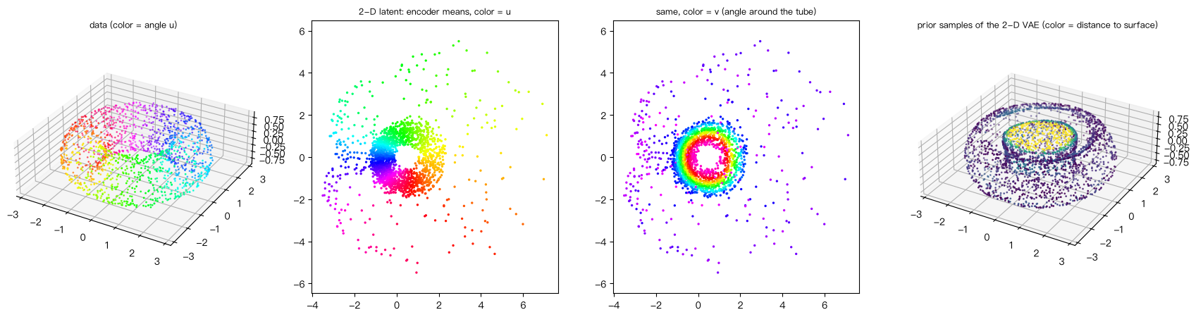
Takeaway. “Interpolating linearly in latent space walks along the data manifold” is a hope, not a theorem. The dimension, the topology and the prior’s shape are all modeling assumptions. Normalizing flows (Lecture 4) cannot even change the dimension, and they meet the same topological wall.
6. VAE vs EM, and K-means
6.1 EM is coordinate ascent on the ELBO
The slides put the VAE next to the classic Expectation–Maximization algorithm (Dempster, Laird & Rubin 1977), which Lecture 2 used to fit patch GMMs. Both maximize the same function ELBO(q, θ):
| how q is chosen | how θ is updated | style | |
|---|---|---|---|
| EM | E-step: q ← p_θ(z | x), the exact posterior, computed analytically | M-step: θ ← argmax ELBO(q, θ), often in closed form | alternate, “max-max” (coordinate ascent) |
| VAE | q_φ(z | x), an encoder network | gradient step on θ | joint stochastic gradient ascent on (θ, φ) |
The slides contrast this with the GAN of Lecture 9, which plays “max-min”.
Why EM never decreases the likelihood. The whole proof uses only the identity of §2.1. Let q_t = p_{θ_t}(z | x) be the E-step result. Then:
- The first inequality holds because the ELBO is a lower bound for any q.
- The second holds because the M-step maximizes over θ.
- The equality holds because the E-step made the KL zero.
Nothing here uses “Gaussian”. EM works whenever the E-step posterior and the M-step maximization are tractable. The VAE exists precisely because, with a neural decoder, neither is.
6.2 Experiment: EM traced step by step
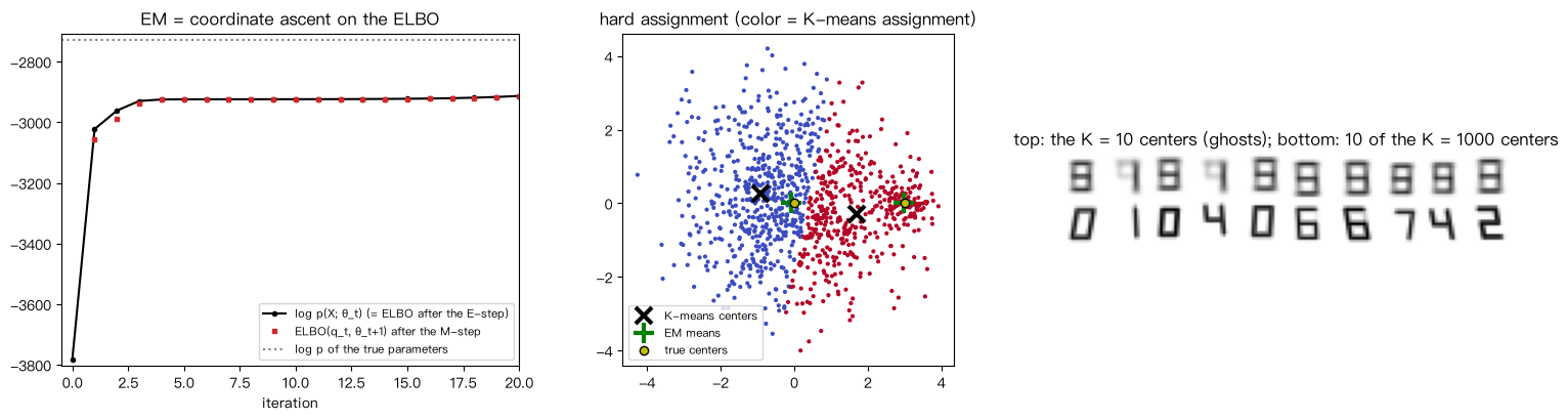
Part 1 of 04_em_and_kmeans.py fits a 3-component GMM to 900 2-D points:
| t | log p(X; θ_t) | ELBO after E | gap | ELBO(q_t, θ_{t+1}) after M | log p(X; θ_{t+1}) |
|---|---|---|---|---|---|
| 0 | −3782.5 | −3782.5 | −4.5e−13 | −3056.6 | −3022.1 |
| 1 | −3022.1 | −3022.1 | 0 | −2987.4 | −2961.0 |
| 5 | −2924.0 | −2924.0 | 0 | −2924.0 | −2923.9 |
| 10 | −2923.7 | −2923.7 | −4.5e−13 | −2923.6 | −2923.6 |
| 20 | −2912.9 | −2912.9 | 0 | −2910.7 | −2908.2 |
| 59 | −2716.8 | −2716.8 | 0 | −2716.8 | — |
Each row shows the chain of inequalities of §6.1 in action:
- after the E-step the gap is zero to machine precision;
- the M-step raises the ELBO;
- the new likelihood is higher still.
The smallest one-step increase over 60 iterations is +2·10⁻⁹: never negative.
But “monotone” does not mean “fast”. With this initialization, two components start almost on top of each other, jointly covering the big left cluster and the upper-right one. The likelihood sits near −2924 for more than ten iterations while they slowly separate (a near-symmetric saddle), and then jumps to −2716.8. That is above the log-likelihood of the true parameters (−2728.6), as maximum-likelihood fits on finite samples should be. EM guarantees no decrease, not the global optimum and not speed; in practice one runs several initializations.
6.3 K-means is EM with variance going to zero
Take a GMM whose K components all have covariance σ²I and equal weights. The E-step responsibilities are a softmax of negative squared distances:
The soft assignment becomes a hard one. The M-step μ_k = Σ_n r_nk x_n / Σ_n r_nk becomes “the mean of the points assigned to k”. That is exactly Lloyd’s K-means algorithm, and the ELBO becomes −(1/2σ²) Σ_n ‖x_n − μ_{k(n)}‖² + const — the K-means objective.
Part 2 of 04_em_and_kmeans.py fixes two K-means centers and computes the responsibilities for decreasing σ. The mean entropy of the responsibilities falls from 0.58 nat (σ = 2) to 0.001 (σ = 0.05), where 99.8% of points are hard-assigned.
The limit has a price. K-means implicitly assumes all clusters are equally wide and equally likely: its decision boundary is the perpendicular bisector of the centers. The script tests this on data with one big wide cluster (900 points, std 1.41, center (0, 0)) and one small narrow one (100 points, std 0.39, center (3, 0)):
| method | center 1 | center 2 | points in cluster 2 |
|---|---|---|---|
| truth | (0.00, 0.00) | (3.00, 0.00) | 100 |
| K-means | (−0.92, +0.25) | (+1.70, −0.30) | 442 |
| EM (own covariances and weights) | (−0.08, +0.01) | (+2.98, +0.02) | 105 (expected) |
K-means hands the outskirts of the big cluster to the small one and drags its center halfway across.
6.4 K-means is an autoencoder, and a bad generative model
The slides make a striking point: K-means is an autoencoder.
- The encoder maps x to the index of its nearest center: a code of log₂K bits.
- The decoder looks the center up.
- The training loss is the reconstruction error.
Read as a generative model (“sample a center with probability ∝ its cluster size”), it is the σ → 0 GMM — a mixture of delta functions. Part 3 of 04_em_and_kmeans.py runs it on 10,000 glyph images:
| K | code length | test reconstruction RMSE | distinct images in 2000 samples | recognizable | mini FID | nearest training image |
|---|---|---|---|---|---|---|
| 10 | 3.3 bit | 0.177 | 10 | 0.068 | 650 | 0.100 |
| 100 | 6.6 bit | 0.137 | 100 | 0.640 | 153 | 0.077 |
| 1000 | 10.0 bit | 0.103 | 824 | 0.915 | 14.5 | 0.054 |
(For comparison, the 8-D VAE reconstructs with RMSE 0.029.)
Two failure modes, at the two ends of K:
- Small K: each center is the average of thousands of different images — a ghost (Lecture 1 §2) that the judge recognizes 7% of the time.
- Large K: each center averages a handful of near-identical training images. The samples look great (FID 14.5, better than any VAE in this lecture!), but there are only 824 distinct ones. They sit closer to training images (0.054) than fresh real images do (0.064). This is memorization, and FID cannot see it (P2 §5).
Adding Gaussian noise to the centers (an isotropic GMM with the within-cluster variance) only sprinkles speckle over the images. The variation of glyph images — shifts, slants, thicknesses — is nothing like “a center plus independent pixel noise”.
How do we keep what is good about K-means — discrete codes, a simple loss — and fix what is bad? Two changes:
- Do the clustering in a learned space. Pixel space is a terrible space for distances.
- Describe each image with many codes instead of one. K^16 combinations instead of K centers.
That is VQ-VAE.
7. VQ-VAE · Discrete latents and the birth of the tokenizer
7.1 The model
VQ-VAE (van den Oord, Vinyals & Kavukcuoglu 2017) keeps the encoder and decoder of a VAE but makes the latent discrete. In order:
- The encoder maps the image to a grid of vectors z_e ∈ ℝ^D. Our code uses 16 vectors on a 4×4 grid, each responsible for a 4×4-pixel patch.
- Quantization. Each vector is replaced by the nearest of K learned code vectors (the codebook e_1, …, e_K): z_q = e_k with k = argmin_j ‖z_e − e_j‖.
- The decoder reconstructs the image from the grid of chosen codes.
So an image becomes a grid of tokens — integers in {1, …, K} — exactly like a sentence is a sequence of word tokens. This is why VQ-VAE and its descendants are called tokenizers (Lecture 7).
7.2 The loss: reconstruction + K-means + commitment
- The codebook loss moves the chosen code toward the encoder output. Averaged over all vectors assigned to code k, its minimizer is their mean — the M-step of K-means, which is why the slides call it a K-means loss used as a regularizer.
- The commitment loss does the opposite: it keeps the encoder outputs near their codes, so the encoder does not drift off and keep “switching” codes.
- The stop-gradients sg[·] keep the two roles separate.
Why is there no KL term? The paper treats the posterior as deterministic, q(z = k | x) = 1 for the nearest code, and the prior during training as uniform over K codes. Then KL(q ‖ p) = log K per token: 16 · log 512 = 99.8 nat per image in our setting. That is a constant, so it is dropped.
7.3 The straight-through gradient
The argmin has no useful gradient: an infinitesimal change in z_e either leaves the chosen code unchanged or jumps to another. VQ-VAE uses the straight-through estimator (Bengio et al. 2013; P1 §5.4):
In the forward pass this equals z_q. In the backward pass the stop-gradient term vanishes, so ∂L/∂z_e = ∂L/∂z_q: the decoder’s gradient is copied straight to the encoder, as if quantization were the identity. Part 1 of 05_vq_vae.py checks both properties, with differences of exactly 0. It also checks that the reconstruction loss gives the codebook no gradient at all: the codebook learns only through the codebook loss. P1 §5.4 showed that straight-through is biased. It works here because z_q stays close to z_e, which is exactly what the commitment loss enforces.
7.4 Experiment: codebook size and dead codes
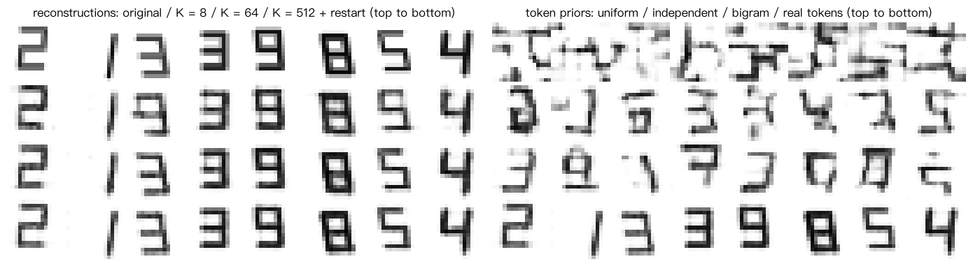
Part 2 of 05_vq_vae.py trains VQ-VAEs with D = 8, 16 tokens per image and 3000 steps:
| setting | bits per image | test RMSE | codes used | perplexity |
|---|---|---|---|---|
| continuous AE (no quantization) | — | 0.026 | — | — |
| K = 8 | 48 | 0.084 | 8 / 8 | 7.7 |
| K = 64 | 96 | 0.054 | 64 / 64 | 43.0 |
| K = 512 | 144 | 0.053 | 104 / 512 | 58.3 |
| K = 512 + dead-code restart | 144 | 0.043 | 512 / 512 | 306.8 |
(Perplexity = exp of the entropy of the code-usage frequencies; K if all codes are used equally.)
Going from K = 64 to K = 512 barely helps — because 408 of the 512 codes are never used. The original implementation initializes the codebook as a tiny cloud U(−1/K, 1/K) around the origin. The encoder outputs are far from all codes, the nearest one is usually one of the same small group, and the rest are never chosen. A code that is never chosen receives no codebook gradient, so it never moves: a dead code.
The fix used here is to restart dead codes: every 200 steps, move each unused code onto a random recent encoder output. This revives all 512 codes and improves the reconstruction to RMSE 0.043. Other standard fixes are k-means initialization of the codebook and exponential-moving-average codebook updates (used in VQ-VAE-2 and later). Lecture 7’s FSQ and LFQ remove the lookup table altogether and make the problem disappear.
7.5 Experiment: a tokenizer is not a generator
Once images are 16 tokens, how do we generate a new one? The slides’ answer: we need a second model for the joint distribution of the tokens — autoregressive (the original paper used a PixelCNN, Lectures 5–6), masked (Lecture 7) or diffusion (Lectures 8, 15). Part 3 of 05_vq_vae.py shows why, decoding token grids from four “priors”:
| token prior | recognizable | valid | mini FID |
|---|---|---|---|
| every token uniformly random | 0.521 | 0.000 | 400 |
| each position independent, from its own frequencies | 0.588 | 0.016 | 266 |
| raster-order bigram (looks at the previous token) | 0.674 | 0.052 | 166 |
| tokens of real test images (the ideal prior) | 0.994 | 0.983 | 5.2 |
Tokens drawn independently decode into fragments from different glyphs glued together. Note the first column: the classifier calls half of these fragment collages “recognizable” with ≥ 90% confidence. This is why the judge also reports a valid rate that requires the image to be close to some real image. A bigram that looks at one previous token helps a little; the real token grids are near perfect. The tokens of one image depend on each other strongly — the strokes must connect, the style must be consistent across the whole digit — and modeling that dependency is the generative problem. The tokenizer only made it discrete and short (16 symbols instead of 256 pixels).
7.6 Why VQ-VAE mattered
VQ-VAE turned generation into a two-stage pipeline:
- Compress. An autoencoder maps images to short sequences of discrete tokens and back. It is trained only for reconstruction (later with perceptual and adversarial losses: VQ-GAN, Lecture 9).
- Generate. A separate model learns the distribution of token sequences.
The second stage can borrow everything from language modeling. This is how DALL·E (2021), Parti and MaskGIT generate images, and why Lecture 7 asks “is the tokenizer the key?”. Continuous latents followed the same two-stage pattern: the VAE in latent diffusion models has a tiny KL weight and serves only as the compressor, while the diffusion model is the generator.
8. The big picture
8.1 The VAE in the five-component framework of Lecture 1
| component | VAE | VQ-VAE (+ token prior) |
|---|---|---|
| formulation | z ~ N(0, I), x ~ p_θ(x | z); variational posterior q_φ(z | x) | x ↦ grid of discrete tokens; separate model of p(tokens) |
| representation | MLP / conv encoder and decoder | encoder, codebook, decoder; AR / masked / diffusion prior |
| objective | ELBO = reconstruction − KL (a lower bound of the likelihood) | reconstruction + codebook + commitment; prior trained by likelihood |
| optimization | SGD with the reparameterization trick | SGD with straight-through; dead-code tricks |
| inference | z ~ p(z), decode (one network pass); density only as a bound (ELBO / IWAE) | sample tokens from the prior, decode |
8.2 Why VAE samples are blurry
Three reasons, which this lecture has measured:
- The Gaussian decoder is an L2 loss. Given z, the decoder predicts the mean of the plausible images (§4.2). Any uncertainty that z does not resolve becomes blur — the ghosts of Lecture 1 §2.
- The prior has holes. Prior samples land in regions the decoder was never trained on (§5.4).
- ELBO training simplifies the model. It prefers decoders whose posteriors the encoder can approximate (§3.3).
Fixes attack each one:
- perceptual and adversarial decoder losses (VQ-GAN, Lecture 9);
- learned priors (VQ-VAE + AR, latent diffusion);
- richer posteriors (normalizing flows in q, Lecture 4; IAF, Lecture 6);
- hierarchical latents (NVAE, VDVAE).
8.3 What survives
The VAE is rarely used as a stand-alone image generator today, but three of its ideas are everywhere:
- The ELBO. It returns as the training objective of diffusion models (Lecture 12), which are hierarchical VAEs with a fixed encoder.
- The reparameterization trick. It is in every model that backpropagates through sampling.
- The encoder–decoder compressor. It is the first stage of nearly every modern image and video generator (Lectures 7, 8, 19).
9. Summary
- A latent-variable model p_θ(x) = ∫ p(z) p_θ(x | z) dz with a neural decoder is expressive, but its likelihood (an integral) and its posterior (which needs that integral) are intractable.
- For any q: log p(x) = ELBO(q) + KL(q ‖ p(z | x)). Maximizing the ELBO over q pulls q toward the posterior; maximizing it over θ pushes the likelihood up. Verified exactly to 10⁻¹¹.
- Because the ELBO contains the reverse KL, a Gaussian q facing a bimodal posterior covers one mode (gap ≈ log 2); the moment-matched Gaussian is far worse.
- Amortization adds a second gap; in our toy it hides in rare inputs (median 0.003 nat, but the worst 1% hold 86%). Training θ with the ELBO biases the model toward Gaussian-friendly posteriors (θ = 0.25 instead of 0.20).
- VAE objective = reconstruction − KL. Gaussian decoder ⇒ L2 with weight 1/(2σ²), so σ acts as β. Diagonal Gaussian vs N(0, I) ⇒ closed-form KL. The reparameterization trick makes the sampling differentiable. Analytic vs sampled KL barely changed the gradient variance here (−0.6%).
- σ (β) trades rate against distortion: dimensions switch off one by one, and at σ = 1.6 the posterior collapses completely. Sample quality peaks in between (σ ≈ 0.4).
- The KL acts per image; the aggregated posterior q(z) still differs from the prior. Prior samples landing in “holes” decode worse (valid rate 0.31 vs 0.83 by emptiness quartile); aggregated-posterior samples are near perfect. A 2-D latent encodes what the pixel loss cares about (translation), not digits.
- The latent’s dimension, topology and prior shape are assumptions: a 2-D VAE turns a torus into an annulus with a seam; a 3-D VAE has no seam but its ball-shaped prior puts 72% of samples off the surface.
- EM is coordinate ascent on the same ELBO with an exact E-step; its monotonicity proof is three lines. K-means is its σ → 0 limit, biased by its equal-width assumption, and it is also an autoencoder whose samples are either ghosts or memorized copies.
- VQ-VAE = clustering in a learned space with many tokens per image; codebook loss = K-means, commitment loss keeps the encoder close, straight-through passes gradients. Dead codes need fixes. A tokenizer still needs a model of the joint distribution of its tokens — the topic of the next five lectures.
10. Common pitfalls
- “The ELBO is an approximation of the likelihood, so maximizing it is maximizing the likelihood.” Only up to the gap, and the gap depends on θ. Training with the ELBO changes which model you learn (§3.3).
- “Use the moment-matched Gaussian as the approximate posterior.” Under the reverse KL of the ELBO this is one of the worst choices for a multimodal posterior (§2.3).
- Forgetting that the decoder σ is a hyperparameter. “MSE + KL” silently fixes β = 2σ² for some σ. Changing the pixel scale (0–1 vs 0–255) or summing instead of averaging over pixels changes the effective β by orders of magnitude.
- Measuring posterior collapse by the total KL only. Look at the KL per dimension: a VAE can have a healthy total KL with most dimensions dead (§4.6).
- Expecting digit clusters in a 2-D latent. The latent encodes what the loss rewards; on our data, that is translation (§5.2).
- Assuming linear interpolation in latent space follows the data manifold. It does only if the latent space and the prior have a compatible shape (§5.5).
- Treating K = 512 as “512 codes”. Check the usage: with a bad initialization only 104 were alive (§7.4).
- Judging a generator by a classifier alone. Half of the random-token collages were “recognizable”; combine several metrics, and look at samples.
- Calling K-means “a generative model with good FID” without checking memorization. FID 14.5 came from 824 near-copies of training images (§6.4).
11. Exercises
1. ELBO via Jensen. Derive ELBO ≤ log p(x) using Jensen’s inequality instead of the KL identity. When is Jensen’s inequality tight, and how does that match the KL identity?
Answer
log p(x) = log ∫ q(z) [p(x, z)/q(z)] dz = log E_q[p(x,z)/q(z)] ≥ E_q[log p(x,z)/q(z)] = ELBO, because log is concave. Jensen is tight iff the random variable p(x, z)/q(z) is constant in z (q-almost surely). That means q(z) ∝ p(x, z), i.e. q(z) = p(z | x) — exactly when the KL term of the identity is zero. The KL identity is more informative because it tells you the size of the gap.
2. The closed-form KL. Derive KL(N(μ, diag σ²) ‖ N(0, I)) = ½ Σ_j (μ_j² + σ_j² − 1 − log σ_j²). Then generalize to KL(N(μ₁, σ₁²) ‖ N(μ₂, σ₂²)) in one dimension.
Answer
Per dimension: KL = E_q[log q − log p] = E_q[−½ log 2πσ² − (z−μ)²/2σ² + ½ log 2π + z²/2] = −½ log σ² − ½ + ½(μ² + σ²). Sum over independent dimensions. General case: KL = log(σ₂/σ₁) + (σ₁² + (μ₁ − μ₂)²)/(2σ₂²) − ½ (P1 §2.3).
3. σ and β. Show that maximizing the ELBO with a Gaussian decoder of fixed variance σ² is equivalent to minimizing E_q‖x − f(z)‖² + β KL(q(z|x) ‖ p(z)) with β = 2σ². In 03_sgvb_and_kl.py, which σ corresponds to β = 1 in the “MSE + KL” form if the MSE is summed over the 256 pixels? And if it is averaged over pixels?
Answer
Multiply the negative ELBO by 2σ²: 2σ² · [‖x − f‖²/(2σ²) + KL] + const = ‖x − f‖² + 2σ² KL + const. So β = 2σ². With a summed MSE, β = 1 ⇔ σ = 1/√2 ≈ 0.71 — between our σ = 0.4 and 0.8, a nearly collapsed regime. With an averaged MSE the reconstruction term is 256 times smaller, which is equivalent to β = 256 in summed form, i.e. σ ≈ 11: complete collapse. This is a classic bug: averaging over pixels while using the standard KL weight.
4. Reparameterization for other distributions. Give a reparameterization for (a) z ~ N(μ, Σ) with full covariance, (b) z ~ Exponential(λ), (c) z ~ Bernoulli(p). Which one fails, and what does VQ-VAE do instead?
Answer
(a) z = μ + Lε with Σ = LLᵀ (Cholesky), ε ~ N(0, I).
(b) z = −log(u)/λ with u ~ Uniform(0, 1): inverse-CDF sampling, differentiable in λ.
(c) Fails: z = 1[u < p] is a step function of p with zero gradient almost everywhere. Options are the score-function estimator, Gumbel-softmax (a continuous relaxation), or straight-through. VQ-VAE uses straight-through on a deterministic nearest-neighbour choice (P1 §5.4).
5. EM monotonicity. Prove log p_{θ_{t+1}}(x) ≥ log p_{θ_t}(x) for EM. Then explain why “generalized EM”, where the M-step only increases the ELBO (e.g. one gradient step) instead of maximizing it, still never decreases the likelihood.
Answer
The chain is log p_{θ_{t+1}} ≥ ELBO(q_t, θ_{t+1}) ≥ ELBO(q_t, θ_t) = log p_{θ_t}:
- the first step holds because the ELBO is a lower bound;
- the second holds because of the M-step;
- the last holds because the E-step makes the KL zero.
The middle inequality only needs the M-step not to decrease the ELBO, so any improving step suffices.
6. K-means as a limit. For a GMM with covariances σ²I and equal weights, show that as σ → 0 the E-step becomes the K-means assignment and the M-step the K-means update. What happens to the ELBO, and why do we say K-means “minimizes the ELBO’s reconstruction term”?
Answer
The responsibilities r_nk = softmax_k(−‖x_n − μ_k‖²/2σ²) converge to the indicator of the nearest center as σ → 0. The M-step then averages the assigned points. The ELBO becomes −(1/2σ²) Σ_n ‖x_n − μ_{k(n)}‖² − nd log σ + const. The entropy of q is 0 for hard assignments, and the log-weight terms are constant. Maximizing it is minimizing the K-means objective (the squared reconstruction error of the “autoencoder” x ↦ μ_{k(x)}).
7. ELBO surgery. Prove E_{p_data(x)}[KL(q(z|x) ‖ p(z))] = I_q(x; z) + KL(q(z) ‖ p(z)), where q(x, z) = p_data(x) q(z|x) and q(z) is its z-marginal. What does this say about a VAE whose KL term is exactly zero?
Answer
E_x KL(q(z|x) ‖ p(z)) = E_{q(x,z)}[log q(z|x) − log p(z)] = E[log q(z|x) − log q(z)] + E[log q(z) − log p(z)] = I_q(x; z) + KL(q(z) ‖ p(z)). Both terms are ≥ 0. If the average KL is zero, both vanish: I_q(x; z) = 0, so z carries no information about x — total posterior collapse, as at σ = 1.6 in §4.6.
8. The torus. (a) Explain why no continuous injective map exists from a torus into the plane, and what that forces a continuous encoder to do. (b) The trained 2-D VAE kept u (the big circle) as a loop and cut v (the tube) open at v ≈ 2.1. Cutting u instead would also give an annulus. Compute the length of the seam in both cases. Does “the encoder minimizes the seam length” explain the choice?
Answer
(a) A torus is a compact surface without boundary. A continuous injective map from it into ℝ² would be open (invariance of domain), so its image would be open and compact, i.e. both open and closed in ℝ² — impossible for a non-empty bounded set. So a continuous encoder must either fold (send distinct points to the same code) or stretch extremely fast somewhere (an approximate tear). Our encoder does the second: it cuts one loop, turning the torus into an annulus (loop × interval), which does embed.
(b) Cutting u at u₀ leaves the seam {u = u₀}, a small circle around the tube of length 2πr = 2π·0.8 ≈ 5.0. Cutting v at v₀ leaves {v = v₀}, a circle around the big axis of length 2π(R + r cos v₀). That is at least 2π(R − r) ≈ 7.5, and ≈ 2π·1.6 ≈ 10.0 at the learned v₀ ≈ 2.1. So “shortest seam” would predict cutting u — the opposite of what happened. The choice is not forced by theory.
A plausible reason is the geometry of the annulus. Keeping the big circle as the angular coordinate and laying the short tube loop along the radius gives a thin ring that resembles a Gaussian blob with a hole. The other choice would put a long loop of radius 2 along the radial direction, a much thicker, more distorted annulus. But this is a hypothesis, not a theorem. Train with other seeds and see whether the seam moves.
9. VQ-VAE’s missing KL. Show that with a deterministic one-hot posterior and a uniform prior over K codes, KL(q ‖ p) = log K for each token. If, after training, you fit a learned prior p_ψ(tokens) (e.g. an autoregressive model), how does the bound on log p(x) change, and what does that tell you about training the prior by maximum likelihood on the encoder’s tokens?
Answer
KL = Σ_k q(k) log(q(k)/p(k)) = 1 · log(1/(1/K)) = log K. With a learned prior, the KL term becomes −log p_ψ(tokens(x)) (the entropy of the one-hot q is 0). The bound is log p(x) ≥ log p(x | tokens) + log p_ψ(tokens(x)). Maximizing the bound over ψ is exactly maximum-likelihood training of the prior on the encoder’s token sequences. The two-stage recipe (train the tokenizer, then fit a prior by MLE on its tokens) is coordinate ascent on one ELBO.
12. Further reading
From the lecture
- D. P. Kingma & M. Welling, Auto-Encoding Variational Bayes, ICLR 2014. D. J. Rezende, S. Mohamed & D. Wierstra, Stochastic Backpropagation and Approximate Inference in Deep Generative Models, ICML 2014.
- A. P. Dempster, N. M. Laird & D. B. Rubin, Maximum Likelihood from Incomplete Data via the EM Algorithm, JRSS-B 1977.
- A. van den Oord, O. Vinyals & K. Kavukcuoglu, Neural Discrete Representation Learning (VQ-VAE), NeurIPS 2017. A. Razavi, A. van den Oord & O. Vinyals, Generating Diverse High-Fidelity Images with VQ-VAE-2, NeurIPS 2019.
- D. P. Kingma & M. Welling, An Introduction to Variational Autoencoders, Foundations and Trends in ML, 2019 (the best long reference).
On the gaps, collapse and the latent space
- Y. Burda, R. Grosse & R. Salakhutdinov, Importance Weighted Autoencoders, ICLR 2016 (IWAE, active units).
- C. Cremer, X. Li & D. Duvenaud, Inference Suboptimality in Variational Autoencoders, ICML 2018 (approximation vs amortization gap).
- R. E. Turner & M. Sahani, Two problems with variational expectation maximisation for time-series models, 2011 (the bias of variational learning).
- M. D. Hoffman & M. J. Johnson, ELBO surgery, NIPS Workshop 2016. S. Zhao, J. Song & S. Ermon, InfoVAE, AAAI 2019. A. Makhzani et al., Adversarial Autoencoders, 2016.
- A. Alemi et al., Fixing a Broken ELBO, ICML 2018 (rate–distortion). I. Higgins et al., β-VAE, ICLR 2017.
- S. R. Bowman et al., Generating Sentences from a Continuous Space, CoNLL 2016; X. Chen et al., Variational Lossy Autoencoder, ICLR 2017 (posterior collapse with strong decoders).
- P. Ghosh et al., From Variational to Deterministic Autoencoders, ICLR 2020 (RAE: AE + post-hoc density).
- Y. Bengio, N. Léonard & A. Courville, Estimating or Propagating Gradients Through Stochastic Neurons, 2013 (straight-through).
In this repository
- Prerequisite P1 §2.3 (Gaussian KL), §4.3 (ELBO and IWAE), §5 (gradient estimators, straight-through, Gumbel-softmax).
- Lecture 1 §2 (ghosts and why regression averages), §4 (latent world models), §5.3 (forward vs reverse KL).
- Lecture 2 §3 (patch GMMs fitted with EM).
13. Next lecture
Lecture 4: Normalizing flows (reading session, 09/17).
The VAE gave up exact likelihoods in exchange for a flexible decoder: its density is only available as a bound, and its posterior only as an approximation. Normalizing flows go the opposite way: make the generator invertible, so that the change-of-variables formula (P1 §6) gives the exact likelihood and the exact “encoder” for free. We will read three papers:
- Rezende & Mohamed (2015) use flows to make the VAE’s q more flexible — a direct answer to §2.3’s mode problem.
- Glow (2018) builds image-scale flows from affine coupling layers and invertible 1×1 convolutions.
- Invertible ResNets (2019) show that ordinary residual networks become invertible when their residual branch is a contraction.
We will also see what flows pay for exactness: the dimension cannot change, and topology (§5.5) becomes a hard constraint.