Prerequisite P1 · Probability, Information & Maximum Likelihood

Role: This lecture does not correspond to any session of the original course. The original prerequisites are a deep-learning course (MIT 6.S898 / 6.7960) plus either computer vision or NLP, and students are assumed to know probability and information theory. Kaiming He’s slides use the KL divergence, the ELBO, reparameterization, Jensen’s inequality and the JS divergence directly when deriving VAEs, GANs and diffusion models. This lecture fills in the probability and information-theory tools that the main lectures actually use, and marks where each one first appears. Basis: The content is standard probability and information theory (see Cover & Thomas, Elements of Information Theory, and Murphy’s Probabilistic Machine Learning, volumes 1 and 2). The examples and experiments were designed for this course. The VAE regularizer formula of §2.3 is problem 3 of the original Pset 1; the ELBO identity of §4.3 is the core of Lecture 3; the bits/dim conversion and dequantization of §7 follow Theis, van den Oord & Bethge (2016). Code: code/prereq1/ (7 scripts; numpy + PyTorch (CPU) + matplotlib; each under 6 seconds) When to read: Before or together with Lecture 1; at the latest before Lecture 3 (VAE). About 4 hours including running the code.

0. How to read this lecture

0.1 Why this lecture

Almost every objective in this course is written in the language of probability and information theory:

If you already know a section, just run its script and glance at the “Observations” to make sure nothing surprises you.

0.2 Learning goals

1. Compute marginals, conditionals and Bayesian posteriors fluently from a joint table; understand that the chain rule “holds in any order, with no approximation”; distinguish independence from conditional independence.
2. Sample a multivariate Gaussian by reparameterization; write the conditional of a multivariate Gaussian; derive $D_{\text{KL}}(\mathcal{N}(\mu, \operatorname{diag}\sigma^2) \Vert \mathcal{N}(0, I))$; know where the samples of a high-dimensional Gaussian are.
3. Understand entropy, cross-entropy and KL as “code lengths”; derive “maximum likelihood = minimizing KL” and understand how maximum likelihood overfits on finite data; compute mutual information.
4. Estimate expectations by Monte Carlo with an error bar; use importance sampling, choose a proposal and know when it fails; verify $\log p(x) = \text{ELBO} + D_{\text{KL}}(q \Vert p(z \mid x))$ with numbers.
5. Derive and compare the two estimators of “the gradient of an expectation” (score function, reparameterization); know why discrete variables are hard and what the straight-through estimator and Gumbel-softmax each pay.
6. Use the change-of-variables formula to get the density after an invertible map; understand why flows prefer triangular Jacobians; understand why “density” does not exist when the dimension is lowered.
7. Convert the negative log-likelihood of a continuous model into bits/dim; understand why dequantization is necessary, and that “likelihood = compression”.

0.3 Map

§1  joint, marginal, conditional; chain rule; independence vs conditional independence; total expectation/variance  ← code 01
§2  Gaussians: reparameterization, conditionals and marginals, the KL between two Gaussians, the soap bubble        ← code 02
§3  information theory: entropy, cross-entropy, KL, maximum likelihood, mutual information, differential entropy  ← code 03
§4  Monte Carlo and importance sampling; the likelihood of a latent-variable model, ELBO, IWAE                       ← code 04
§5  gradients of expectations: score function vs reparameterization; discrete variables                           ← code 05
§6  change of variables; triangular Jacobians; lowering the dimension                                                 ← code 06
§7  bits/dim, dequantization, likelihood = compression                                                                ← code 07
§8  summary   §9 common pitfalls   §10 exercises   §11 further reading

0.4 Notation

1. Joint, marginal, conditional

1.1 A joint probability table

The slides of Lecture 5 (autoregressive models) use a three-variable example: vehicle type $A \in \{\text{car}, \text{bus}\}$, color $B \in \{\text{dark}, \text{light}\}$, age $C \in \{\text{new}, \text{old}\}$. Script 01 makes up probabilities for it, giving a $2 \times 2 \times 2$ joint distribution $p(A, B, C)$ whose 8 entries sum to 1. With the joint, everything else can be computed:

• Marginal: sum over the variables you do not care about. $p(B) = \sum_a \sum_c p(a, B, c)$. Here $p(B = \text{dark}) = 0.48$.
• Conditional: joint divided by marginal. $p(A \mid B) = p(A, B) / p(B)$. Here $p(A \mid B = \text{dark}) = (0.875, 0.125)$.
• Bayes’ rule: “reverse” a conditional, $p(A \mid B) = p(B \mid A)\,p(A) / p(B)$. The two computations in the code give exactly the same numbers. After seeing $C = \text{old}$, $p(A = \text{bus})$ goes from the prior 0.300 to the posterior 0.454 — buses are more often old, and the observation changes the belief.

The hard part is never these formulas but the joint distribution itself. A joint table over $d$ binary variables has $2^d - 1$ free parameters; one 28×28 black-and-white image means $2^{784}$ numbers. All the effort of generative modeling goes into representing this table without writing it down (the “factorizations” of Lecture 1 §6).

1.2 The chain rule: any order, no approximation

Applying the definition of a conditional $p(A, B) = p(A)\,p(B \mid A)$ repeatedly gives the chain rule:

Part 2 of script 01 factorizes the same table in all 6 orders (A→B→C, A→C→B, …), multiplies the factors back, and gets the original table to within $10^{-17}$ (floating-point rounding). Two things to remember:

1. The chain rule holds for any order, with no approximation. So an autoregressive model may generate in any order (Lecture 5; MAR in Lecture 8 exploits “any order”). The approximation only enters through “what we use to represent each conditional”.
2. The data were generated A → B → C, but that does not make other orders “untrue”. A factorization is a modeling choice, not a causal claim. (Different orders can still be easier or harder to learn — the unimodal-Gaussian example of Lecture 1, script 06.)

1.3 Independence and conditional independence

• Independence: $p(x, y) = p(x)\,p(y)$, equivalently $p(x \mid y) = p(x)$ — knowing $y$ does not help you guess $x$.
• Conditional independence: given $z$, $p(x, y \mid z) = p(x \mid z)\, p(y \mid z)$.

Neither implies the other. Part 3 of script 01 shows both directions:

(a) Independent causes become dependent through a common effect (“explaining away”). Rain $R$ (20%) and a sprinkler $S$ (30%) are independent; wet grass $W \approx R \lor S$.

Seeing wet grass makes rain more likely; learning that the sprinkler was on brings rain back to its prior — the sprinkler “explains away” the wet grass. Given the common effect $W$, the originally independent $R$ and $S$ become dependent.

(b) Dependent observations become independent given a common latent. Let $z$ mean “this is a 0 or a 1”; given $z$, two pixels $x_1$, $x_2$ turn on independently with probability $q_z$ ($q_0 = 0.1$, $q_1 = 0.9$):

This is the central trick of latent-variable models:

Each $p(x_i \mid z)$ is extremely simple (pixels independent), but after summing (or integrating) over $z$, the components of $x$ have rich dependencies. The decoder of the Lecture 3 VAE outputs “an independent Gaussian per pixel”, yet the whole model represents complex correlations between pixels — for exactly this reason. GlyphWorld in Lecture 1 §4.2 works the same way: given all 7 latents the image is determined; without them the pixels have long-range correlations.

1.4 The laws of total expectation and total variance

Part 4 of script 01 checks this on a mixture of three Gaussians: sample mean −0.1037 (formula −0.1000), sample variance 4.3573 (formula 0.28 + 4.09 = 4.37), with Monte Carlo error as the only difference. The law of total variance has exactly the shape of the mean-squared-error decomposition of Lecture 1 §2.3: regression can only remove the “between” part; $\mathbb{E}[\operatorname{Var}(X \mid Y)]$ is a floor that no regression can go below — and a generative model’s job is precisely to represent that remaining uncertainty instead of averaging it away.

2. The Gaussian

2.1 Density and reparameterization

The density of a $d$-dimensional Gaussian $\mathcal{N}(\mu, \Sigma)$ is

Reparameterization: every Gaussian can be written as “a standard normal + a deterministic transformation”:

Part 1 of script 02 checks this with 200,000 samples: the largest difference between the sample covariance and the target is 0.0022. The point of reparameterization: all randomness is in $\epsilon$, and the parameters $\mu$, $L$ appear only in the deterministic part, so we can differentiate through the sample (§5). The log density is computed with the Cholesky factor too: the quadratic form $= \Vert L^{-1}(x-\mu) \Vert^2$ and $\log|\Sigma| = 2\sum_i \log L_{ii}$, more stable than an explicit inverse.

2.2 Marginals, conditionals, the linear-Gaussian model

Split $x$ into two blocks $(x_1, x_2)$, with the mean and covariance split accordingly:

• Marginal: $x_1 \sim \mathcal{N}(\mu_1, \Sigma_{11})$ (just take the block).
• Conditional: $x_1 \mid x_2 \sim \mathcal{N}\big(\mu_1 + \Sigma_{12}\Sigma_{22}^{-1}(x_2 - \mu_2),\ \Sigma_{11} - \Sigma_{12}\Sigma_{22}^{-1}\Sigma_{21}\big)$.

The conditional mean is a linear function of the observation $x_2$; the conditional covariance does not depend on the observed value and is always smaller than the marginal covariance (knowing $x_2$ reduces uncertainty). Part 2 of script 02 takes samples in a thin slice around $x_2 = 2$: mean 0.395, variance 0.693, against the formula’s 0.400 and 0.680 (the small variance difference comes from the slice’s width). A conditional is “a slice of the joint along a line, renormalized”:

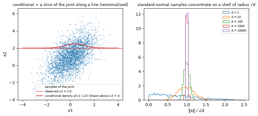
A linear-Gaussian latent-variable model: $z \sim \mathcal{N}(0, 1)$, $x \mid z \sim \mathcal{N}(az, s^2)$. $(z, x)$ is jointly Gaussian, so the marginal $p(x) = \mathcal{N}(0, a^2 + s^2)$ and the posterior $p(z \mid x)$ have closed forms (precisions add: $1/\sigma_{\text{post}}^2 = 1 + a^2/s^2$, $\mu_{\text{post}} = \sigma_{\text{post}}^2\, a x / s^2$). With $a = 2$, $s = 0.5$, $x = 1$, samples give a posterior mean 0.4711 and variance 0.0589, the formula 0.4706 and 0.0588. The multivariate version is “probabilistic PCA”. A VAE’s decoder is a nonlinear neural network, and its posterior has no closed form — which is why Lecture 3 approximates the posterior with an encoder $q_\phi(z \mid x)$. §4.3 keeps using this model for experiments, because everything about it can be computed exactly.

2.3 The KL between two Gaussians

The KL divergence (formally defined in §3) between two $d$-dimensional Gaussians has a closed form:

The special case used most in VAEs is a diagonal Gaussian against the standard normal:

This is exactly what problem 3 of the original Pset 1 asks you to prove. The derivation is short. The dimensions are independent, so the KL is a sum over dimensions; in one dimension, $D_{\text{KL}} = \mathbb{E}_q[\log q - \log p] = -\tfrac12\log(2\pi e\sigma^2) + \tfrac12\log 2\pi + \tfrac12\mathbb{E}_q[z^2] = -\tfrac12(1 + \log\sigma^2) + \tfrac12(\mu^2 + \sigma^2)$.

Part 3 of script 02 compares the closed form with Monte Carlo estimates (true KL 0.5531):

Monte Carlo is unbiased but noisy; at $N = 10$ the noise is about as large as the KL itself. Use the closed form wherever it exists — the difference between the “SGVB estimator” and the “analytic KL” ways of training a VAE in the original Pset 1 is exactly this.

The per-dimension contributions have an intuitive meaning. In the example, $\mu = (0.3, -1.2, 0, 2)$ and $\log\sigma^2 = (-1, 0.5, 0, -3)$, and the four dimensions contribute 0.229, 0.794, 0.000 and 3.025:

• the dimension with $\mu = 0$, $\sigma^2 = 1$ contributes exactly 0;
• the further the mean from 0 and the variance from 1, the larger the contribution.

This is what the VAE regularizer does: it “pulls each data point’s code distribution toward the standard normal”.

2.4 The high-dimensional “soap bubble”

Samples of a $d$-dimensional standard normal have norms concentrated around $\sqrt{d}$: $\Vert x\Vert^2 = \sum_j x_j^2$ has mean $d$ and variance $2d$, so $\Vert x \Vert \approx \sqrt{d} \pm 0.7$.

The density at the origin (the mode) is $d/2$ nats higher than at a typical sample, yet no sample is there. The point of highest probability density is not where the probability mass is: mass = density × volume, and the volume of a shell grows rapidly with its distance from the origin. This is the mathematical reason behind pitfall 2 of Lecture 1 (“the best generation is the most probable sample”), and the reason why “noisy images in a diffusion model almost all lie on a shell of radius $\sqrt d$”.

3. Information theory

3.1 Entropy: the average length of the best code

The entropy of a discrete distribution $p$ is

The best way to understand it is through coding. Shannon’s source coding theorem says:

• for symbols from $p$, no uniquely decodable binary code can have an average length below $H(p)$;
• a code with average length below $H(p) + 1$ always exists;
• ideally, a symbol of probability $p(x)$ should get $-\log_2 p(x)$ bits (the more common, the shorter).

Script 03 checks this with Huffman codes:

Entropy measures “uncertainty”: the uniform distribution is the most uncertain (3 bits), the almost-certain one less than 0.3 bit. When all probabilities are powers of 2, the code lengths equal $-\log_2 p$ exactly. Huffman cannot go below 1 bit per symbol in the “almost certain” row. Encoding many symbols together, or arithmetic coding, approaches the entropy.

3.2 Cross-entropy and KL: the extra bits of the wrong code

Encoding data from $p$ with “the ideal code designed for $q$” (length $-\log_2 q(x)$) takes, on average, the cross-entropy:

The KL divergence is “the extra bits spent because the model is wrong”. Part 2 of script 03 (data from the “skewed” distribution above, $H = 2.1295$):

Three properties:

1. Non-negative: $D_{\text{KL}}(p\Vert q) \ge 0$, with equality iff $p = q$ (by Jensen’s inequality, exercise 2).
2. Asymmetric: $D_{\text{KL}}(p\Vert q) \ne D_{\text{KL}}(q \Vert p)$ (the uniform row; the forward / reverse KL of Lecture 1 §5.3).
3. Support: as soon as $q$ gives probability 0 to a symbol that really occurs, $D_{\text{KL}}(p\Vert q) = \infty$; the other direction can still be small (last row).

3.3 Maximum likelihood = minimizing KL = sample frequencies; and its overfitting

Fit a $K$-class categorical distribution $q = (q_1, \dots, q_K)$ to $N$ samples. The mean log-likelihood is $\frac1N\sum_k n_k \log q_k$ ($n_k$ = how often class $k$ occurs). Maximizing it subject to $\sum_k q_k = 1$ with a Lagrange multiplier gives $\frac{n_k}{N q_k} = \lambda$, i.e.

The maximum-likelihood estimate is the sample frequency. It is also the solution of “minimize $D_{\text{KL}}(\hat p_{\text{data}} \Vert q)$” ($\hat p_{\text{data}}$ = the empirical distribution of the samples), the same derivation as Lecture 1 §5.2.

The trouble is finite data. Part 3 of script 03 uses a 50-class long-tailed distribution (entropy 4.234 bits):

Maximum likelihood gives unseen classes probability 0; as soon as real data contain one, the cross-entropy is infinite. This is overfitting for a probability model, the same thing as the kernel density estimate with bandwidth $h \to 0$ in Lecture 1 §4.5. The simplest remedy is add-$\alpha$ smoothing, $q_k = (n_k + \alpha)/(N + K\alpha)$ (equivalent to putting a prior on the model), with $\alpha$ chosen on a validation set. This “zero-probability disaster” is everywhere in language and pixel models; it comes back with PixelCNN (Lecture 6).

3.4 Mutual information and the data processing inequality

Mutual information measures “how much the uncertainty about $X$ drops once $Y$ is known”:

The second form says that mutual information is “how far the joint is from independence”. Part 4 of script 03 uses a binary symmetric channel: $X$ uniform on 0/1, $Y$ = $X$ flipped with probability $\varepsilon$, $Z$ = $Y$ flipped again with probability $\varepsilon$:

Data processing inequality: if $X \to Y \to Z$ is a Markov chain, then $I(X; Z) \le I(X; Y)$ — no processing of data can create new information. The conditional-entropy table of Lecture 1 §7 asks “how much information about $x$ does the condition $y$ contain”; the forward process of a diffusion model (Lecture 12) is a Markov chain that loses information step by step.

3.5 Continuous variables: differential entropy and the invariance of KL

The “differential entropy” $h(p) = -\int p \log p$ of a continuous variable is not a direct generalization of discrete entropy. A Gaussian’s differential entropy is $\tfrac12\log_2(2\pi e\sigma^2)$. For $\sigma = 2, 1, 0.5, 0.1$ it is +3.05, +2.05, +1.05 and −1.27 bits: it can be negative. Scaling the variable by $a$ adds $\log_2|a|$. It depends on units and coordinates.

The KL divergence, however, is invariant under invertible transformations. Applying the same invertible map $y = g(x)$ to both distributions multiplies both densities by the same Jacobian factor (§6), which cancels in the ratio $p/q$. Part 5 of script 03: $D_{\text{KL}}(\mathcal{N}(0,1) \Vert \mathcal{N}(1, 1.5^2))$ is 0.3499 nat in closed form, estimated as 0.3505 on $x$, and still 0.3505 after the transformation $y = e^x$. So comparisons between models use likelihood differences (or KL), and reporting a single negative log-likelihood of continuous data requires saying how the data were scaled and discretized (§7).

3.6 Preview: “distances” beyond KL

4. Monte Carlo and importance sampling

4.1 Monte Carlo: if you can sample, you can estimate expectations

The estimate is unbiased, its standard deviation is $\sigma_f / \sqrt{n}$, and it does not depend on the dimension of $x$. Part 1 of script 04 estimates $\mathbb{E}[\cos X]$ for $X \sim \mathcal{N}(0,1)$. For $n = 10, 100, 1000, 10000$ the standard deviations are 0.142, 0.044, 0.014 and 0.0046, so “std × $\sqrt n$” stays at about 0.45. The interval “mean ± 1.96 × standard error” contains the truth 94–95% of the time, but only 87% at $n = 10$, where the standard error itself is poorly estimated. Ten times the accuracy costs a hundred times the samples, but the dimension does not matter — which is why all training of generative models is built on “sample + average”.

4.2 Importance sampling

To estimate $\mathbb{E}_p[f]$ when $p$ is hard to sample (or to sample more “where it matters”), sample from another distribution $q$ and reweight:

Even better, when $p$ is known only up to a constant ($p(x) = \tilde p(x)/Z$), we can estimate the normalizing constant: $Z = \int \tilde p = \mathbb{E}_q[\tilde p(x)/q(x)]$. This is the core difficulty of the energy-based models of Lecture 12 ($p(x) \propto e^{-E(x)}$). Part 2 of script 04 uses the double-well energy $E(x) = x^4/4 - x^2$ (true $Z = 7.5875$) and proposals $q = \mathcal{N}(0, s^2)$, with 1000 samples each:

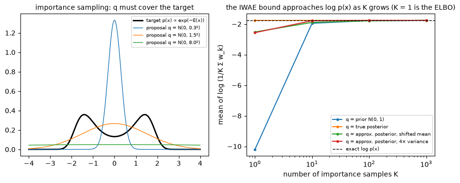
The effective sample size $\text{ESS} = (\sum w_i)^2 / \sum w_i^2$ measures how uneven the weights are. The rule: $q$ must “cover” the target; its tails must not be lighter than the target’s. When $q$ is too narrow, the target’s two valleys are almost never sampled, and the rare hit gets an enormous weight. The estimate is unbiased in theory, but in practice it is almost always too small and occasionally huge. This is the same reason why the forward KL of Lecture 1 “must cover all the data”.

Rare events are the classic use of importance sampling. For $P(X > 4)$ with $X \sim \mathcal N(0,1)$ (truth $3.17\times10^{-5}$):

• plain sampling with 100,000 samples has relative std 52.6%;
• sampling from $\mathcal{N}(4, 1)$ and reweighting has relative std 0.71%.

4.3 The likelihood of a latent-variable model: ELBO and IWAE

How do we compute the likelihood of a latent-variable model $p(x) = \int p(z)\,p(x \mid z)\,dz$? Importance-sample with an approximate posterior $q(z \mid x)$:

Taking the log and using Jensen’s inequality ($\log$ is concave, so $\log \mathbb{E} \ge \mathbb{E} \log$):

And the gap is exactly a KL:

(Proof: substitute $p(x, z) = p(z \mid x)p(x)$ into the ELBO; $\log p(x)$ does not depend on $z$ and comes out, and what remains is $-D_{\text{KL}}$.) This is the central identity of the VAE in Lecture 3. Part 4 of script 04 checks it on the linear-Gaussian model of §2.2, whose $\log p(x) = -1.7600$ is known exactly:

• Columns 3 and 4 agree (up to Monte Carlo error): the gap between the ELBO and the true log-likelihood is the KL from the approximate posterior to the true one.
• When $q$ is the true posterior, every sample’s weight equals $p(x)$ exactly; the estimate has zero variance and the ELBO equals $\log p(x)$. So “maximize the ELBO” does two things at once: it raises the likelihood and pushes $q$ toward the true posterior.
• The IWAE bound $\mathbb{E}\big[\log \frac1K\sum_k w_k\big]$ (average the weights first, then take the log) approaches $\log p(x)$ as $K$ grows; the worse $q$, the larger the $K$ needed. $q$ = prior is the worst — which is why a VAE trains an encoder to approximate the posterior instead of sampling $z$ from the prior. (At $K = 1000$ a few numbers are slightly above $\log p(x)$: IWAE is a lower bound only in expectation, and the average over 200 repeats is still noisy.)

5. Gradients of expectations

5.1 The problem

Generative models often optimize $L(\theta) = \mathbb{E}_{z \sim q_\theta}[f(z)]$: an expectation over a distribution that depends on the parameters. Examples are the ELBO as a function of the encoder’s parameters, a reverse KL, and reinforcement learning. We cannot simply move $\nabla_\theta$ inside the expectation, because the sampling itself depends on $\theta$.

The score-function estimator (also called REINFORCE or the likelihood-ratio estimator) uses the “log-derivative trick” $\nabla_\theta q_\theta = q_\theta \nabla_\theta \log q_\theta$:

It needs only the values of $f$; $f$ need not be differentiable, and discrete variables are fine. Since $\mathbb{E}_q[\nabla_\theta \log q_\theta] = \nabla_\theta \int q_\theta = 0$, any baseline $b$ that does not depend on $z$ can be subtracted from $f$ without changing the expectation. A good baseline can cut the variance dramatically.

The reparameterization estimator (also called pathwise). If $z = g_\theta(\epsilon)$ with the distribution of $\epsilon$ independent of $\theta$ (§2.1), then

It needs $f$ differentiable in $z$ and $z$ differentiable in $\theta$, but it uses the extra information in the derivative of $f$.

5.2 Experiment: variance, baselines and dimension

$L(\mu, \sigma) = \mathbb{E}_{z\sim\mathcal{N}(\mu,\sigma^2)}[(z-2)^2] = (\mu-2)^2 + \sigma^2$ has true gradient $(-4, 2)$ at $\mu = 0$, $\sigma = 1$. With $B = 10$ samples per estimate (part 1 of script 05):

All three are unbiased; reparameterization has a 3–5× smaller standard deviation. The dimension matters even more. Take $f(z) = \Vert z - 2\Vert^2$ and the gradient with respect to $\mu_1$:

In the score-function estimator, the value of $f$ contains the random fluctuations of the other $d-1$ dimensions, and all of it becomes noise. A VAE has tens to hundreds of latent dimensions, so it cannot do without reparameterization (Lecture 3).

5.3 The precondition of reparameterization

Take the step function $f(z) = \mathbb{1}[z > 1]$, so $L = P(z > 1)$, with true gradient $\phi(1) = 0.242$.

• The score-function estimator gives 0.2403 ± 0.0571.
• Reparameterization gives 0.0000 ± 0.0000.

A step function has derivative 0 almost everywhere, and reparameterization “honestly” returns 0 — completely wrong. Reparameterization requires $f$ to be differentiable.

5.4 Discrete variables: straight-through and Gumbel-softmax

A discrete variable $k \sim \text{Categorical}(\operatorname{softmax}(\theta))$ cannot be written as “a continuous, differentiable transformation”, so reparameterization fails. The VQ-VAE of Lecture 3 (a discrete codebook) and DALL·E’s discrete VAE in Lecture 7 both face this problem. Part 4 of script 05 compares several approaches on $L = \mathbb{E}[(v_k - c)^2]$; the exact gradient can be computed by enumeration and has length 0.450.

• The score-function estimator is still unbiased for discrete variables, just noisy.
• The straight-through estimator uses the real discrete sample (a one-hot) in the forward pass and pretends it was the softmax output in the backward pass. In code it is the one line on the Lecture 3 slides, stop_grad(hardmax(y) − softmax(y)) + softmax(y). It is a heuristic: unbiased exactly when $f$ is linear (because $\mathbb{E}[\text{one-hot}] = \text{softmax}$), and more biased the more curved $f$ is. Here its bias (0.61) exceeds the true gradient itself (0.45), and its noise is no smaller than the score function’s. It is good enough in VQ-VAE because only a “roughly correct direction” is needed there and the quantization is a deterministic nearest-neighbour choice.
• Gumbel-softmax. The Gumbel-max trick says that $\arg\max_k(\theta_k + g_k)$, with independent Gumbel noises $g_k$, is distributed exactly as $\operatorname{softmax}(\theta)$. Replacing the argmax with a softmax at temperature $\tau$ gives a differentiable “soft one-hot”. A large $\tau$ is smooth, with low noise and high bias; $\tau \to 0$ approaches true discrete sampling, with low bias and high noise. The temperature trades bias against variance.

6. Change of variables

6.1 One dimension

Let $z \sim p_z$ and $x = g(z)$ with $g$ strictly monotone. The probability that $x$ falls in $[x, x + dx]$ equals the probability that $z$ falls in the corresponding interval $[z, z + dz]$: $p_x(x)|dx| = p_z(z)|dz|$, so

Wherever the map stretches an interval, the density thins out by the same factor. Part 1 of script 06 checks three maps:

• $x = e^z$ (log-normal, $p_x(x) = \phi(\log x)/x$): at $x = 0.3$ the histogram gives 0.6450 and the formula 0.6442.
• $x = \Phi(z)$ (the normal CDF) turns a normal into a uniform distribution (all three histogram values ≈ 1). Conversely, $\Phi^{-1}$ turns a uniform into a normal.
• The non-monotone $x = z^2$ has two preimages $\pm\sqrt{x}$, and the two branches must be added: $p_x(x) = [\phi(\sqrt x) + \phi(-\sqrt x)]/(2\sqrt x)$.

Finding all preimages is almost impossible in high dimensions, so models that want exact likelihoods insist on invertible maps.

6.2 Several dimensions: the Jacobian determinant

For an invertible, differentiable $x = g(z)$ with the $d \times d$ Jacobian $J = \partial g / \partial z$:

$|\det J|$ is “how much $g$ magnifies a small volume”. Part 2 of script 06: for linear maps $x = Az$, the densities of the $\det A = 2.85$ group are all about 2.85 times smaller.

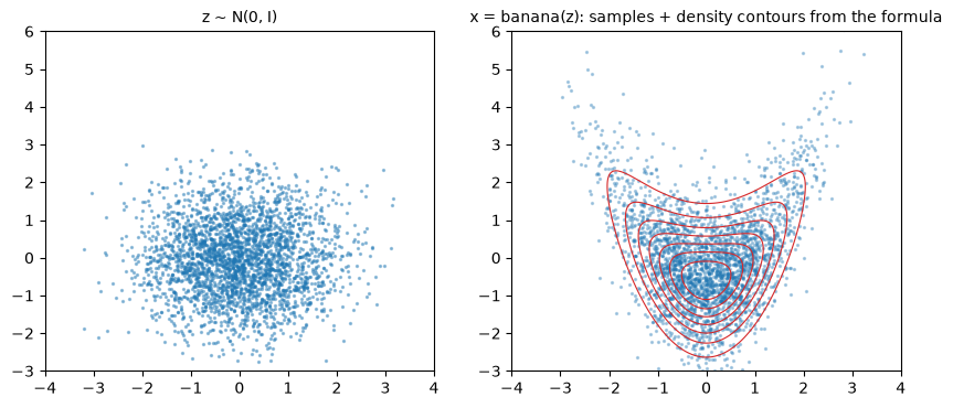
Triangular Jacobians. The banana map $x_1 = z_1$, $x_2 = z_2 + b(z_1^2 - 1)$ is nonlinear, but $x_2$ depends only on $z_2$ and the “earlier” $z_1$. So:

• its Jacobian is lower triangular, $\begin{pmatrix}1 & 0\\ 2bz_1 & 1\end{pmatrix}$;
• its determinant is always 1;
• its inverse is explicit ($z_2 = x_2 - b(x_1^2-1)$).

Histograms and the formula agree (e.g. 0.0851 vs 0.0852). The coupling layers of Lecture 4 and the autoregressive flows (IAF / MAF) of Lecture 6 all have this structure.

6.3 Composition: log-determinants add up

For $x = g_K \circ \cdots \circ g_1(z)$ with every step invertible:

This is the whole secret of normalizing flows. Part 3 of script 06 composes “scale-and-shift → banana → rotation”, inverts step by step and adds the log-determinants; the result agrees with the histogram (e.g. 0.1081 vs 0.1073).

The cost is in the determinant:

• a general $d \times d$ determinant needs $O(d^3)$ (LU factorization);
• a triangular one needs $O(d)$ (the product of the diagonal).

At $d = 1600$ the timings on this machine are about 8 ms vs 0.01 ms. A 256×256 color image has $d \approx 200{,}000$, and the determinant of a general Jacobian is out of reach. The two constraints “invertible + cheap determinant” are the root of the structural limits of normalizing flows (Lecture 4).

6.4 When the dimension drops, the density does not exist

If $g$ maps a low-dimensional $z$ into a higher-dimensional space ($x = (z, 2z)$, $z \in \mathbb{R}$), all samples lie on a straight line. A line has “zero area” in the plane, so the 2-D density is infinite on the line and zero off it — it does not exist. Part 4 of script 06 has to add a small noise $\varepsilon$ to the covariance of a 2-D Gaussian to invert it. As $\varepsilon$ falls from 0.1 to $10^{-8}$, the mean log-likelihood of test samples climbs from −2.00 to +6.06, without limit.

Real images may also concentrate near a low-dimensional manifold (Lecture 1: GlyphWorld has only 7 knobs). Hence:

• a VAE’s decoder outputs a noisy distribution (Lecture 3);
• a normalizing flow keeps the dimension (Lecture 4);
• discrete pixel values must be “dequantized” before a continuous density is computed (§7).

7. Bits per dimension, dequantization and “likelihood = compression”

7.1 Discrete and continuous likelihoods

Pixels are integers 0–255, but models are often continuous densities (flows, VAEs, diffusion). With the data scaled to $[0, 1]$, the integer $k$ corresponds to the interval $[k/256, (k+1)/256)$ of width $\Delta = 1/256$:

Part 1 of script 07: the discrete negative log-likelihood is 6.9815 bits, the continuous density at the bin centers gives −1.0185 bits, and adding 8 gives exactly 6.9815. A continuous “negative log-likelihood” can be negative; only after adding 8 bits does it mean “how many bits to encode one 8-bit pixel”. The bits/dim in papers is

(With data scaled to $[-1, 1]$, $\Delta = 2/256$ and the constant becomes 7 — check the scaling before comparing numbers across papers.) For reference, PixelCNN++ reports about 2.92 bits/dim on CIFAR-10; 8 bits would mean “the model learned nothing”.

7.2 Continuous models cheat on discrete data; dequantization

Fit a continuous density directly to integer data and the model can pile its probability onto the integers, exactly where the test data fall too — the likelihood can be infinite. Part 2 of script 07 (16 gray levels, true entropy 3.337 bits) shows this with a kernel density estimate:

Without dequantization, the smaller the bandwidth, the lower the “negative log-likelihood” — far below the entropy and even negative: cheating. Uniform dequantization (Theis et al. 2016): add uniform noise $u \in [0,1)$ to every integer and train and evaluate the continuous model on $k + u$. By Jensen’s inequality,

so the continuous dequantized NLL is an upper bound on the induced discrete NLL, and cheating is impossible (column 3 ≥ column 4 ≥ entropy). With a too-small bandwidth the bound gets worse again — gaps between training points, overfitting once more. Flow++ (Ho et al. 2019) replaces the uniform noise with a learned “variational dequantization” distribution to tighten the bound.

7.3 Likelihood = compression

§3.1 said that the ideal code gives data of probability $p$ a length of $-\log_2 p$ bits (arithmetic coding achieves this almost exactly). So every probability model is a compression method, and bits/dim is the number of bits per pixel it needs. Part 3 of script 07 compares models on glyph images quantized to 0–255:

Each extra dependency the model captures saves bits:

• (b) treats all pixels alike;
• (c) lets each position have its own distribution;
• (d) makes each pixel depend on its neighbours, and with only two neighbours it already beats zlib.

lzma is better still, because it finds long repeated fragments (the same strokes recur across the 2000 images). Probability models with larger contexts — the PixelCNN of Lectures 5–6 — are needed to go lower. The “negative log-likelihood = cross-entropy” that problem 1 of the original Pset 2 proves is exactly what trains this column.

8. Summary

1. With the joint distribution everything can be computed; the hard part is the joint itself. The chain rule holds exactly in any order; independence and conditional independence do not imply each other; “components independent given a latent” can represent rich correlations — the trick of latent-variable models.
2. Gaussians:
   • reparameterization $x = \mu + L\epsilon$;
   • the conditional mean is linear and the conditional variance does not depend on the observation;
   • the KL between two Gaussians has a closed form (the VAE regularizer $-\tfrac12\sum(1 + \log\sigma^2 - \mu^2 - \sigma^2)$);
   • high-dimensional samples live on a thin shell of radius $\sqrt d$, and the mode is not typical.
3. Information theory:
   • entropy = optimal code length; cross-entropy = entropy + KL;
   • maximum likelihood = minimizing KL = sample frequencies, which on finite data gives unseen events probability 0;
   • mutual information = how far the joint is from independence, and it only decreases along a chain;
   • KL is invariant under invertible maps, differential entropy is not.
4. Monte Carlo is unbiased, its error is $\propto 1/\sqrt n$, and it does not depend on the dimension. An importance-sampling proposal must cover the target. $\log p(x) = \text{ELBO} + D_{\text{KL}}(q \Vert p(z\mid x))$, and the IWAE bound approaches $\log p(x)$ as the number of samples grows.
5. Gradients of expectations:
   • the score-function estimator is general but noisy, and gets worse with dimension;
   • reparameterization has low variance but requires differentiability;
   • for discrete variables, use the score function (unbiased, noisy), straight-through (a biased heuristic) or Gumbel-softmax (the temperature trades bias for variance).
6. Change of variables: $\log p_x = \log p_z - \log|\det J|$, and log-determinants add under composition. Triangular Jacobians turn $O(d^3)$ into $O(d)$. When the dimension drops, the density does not exist.
7. bits/dim = negative log-likelihood per dimension (in bits) + a discretization constant. Continuous models need dequantization on discrete data. Likelihood is compression.

9. Common pitfalls

1. “A probability density cannot exceed 1.” A probability mass function cannot; a density can ($\mathcal N(0, 0.1^2)$ is about 4 at 0). So the “negative log-likelihood” of a continuous model can be negative (§7.1).
2. “The chain rule is an approximation / autoregressive models assume independence.” The chain rule is an identity; the approximation comes from how each conditional is represented (§1.2).
3. “The KL divergence is a distance.” It is asymmetric and violates the triangle inequality (§3.2).
4. “Maximum likelihood is always a good estimator.” On finite data it overfits and gives unseen events probability 0 (§3.3); in the continuous case it can even push the likelihood to infinity (§6.4, §7.2).
5. “Importance sampling is unbiased, so any proposal will do.” Unbiased only in expectation; with a too-narrow proposal the variance can be infinite and the estimate you actually get is almost always too small (§4.2).
6. “A larger ELBO means a better approximate posterior.” ELBO = $\log p(x) - D_{\text{KL}}$ depends both on the model’s likelihood and on the quality of the posterior approximation; the ELBOs of two different models say nothing direct about whose posterior approximation is better (§4.3).
7. “Reparameterization is always better than the score function.” It requires a differentiable $f$ and continuous variables; with a non-differentiable $f$ it gives a wrong gradient (§5.3).
8. “Straight-through gives an approximation of the true gradient.” It is a biased heuristic, and its bias can exceed the gradient itself (§5.4).
9. “Bits/dim can be compared directly across papers.” Check how the data were scaled, discretized and dequantized (§7.1, §7.2).

10. Exercises

Exercise 1 (the parameter count of the chain rule) How many free parameters does the full joint table of $d$ discrete variables with $K$ values each have? What if you use the chain rule with every conditional also stored as a full table? Explain why “the chain rule itself saves no parameters; the savings come from how the conditionals are represented”.

Full joint table: $K^d - 1$. Chain rule with full conditional tables: the $i$-th conditional needs $K - 1$ numbers for each of the $K^{i-1}$ values of $x_{<i}$, for a total of $\sum_{i=1}^d K^{i-1}(K-1) = K^d - 1$ — exactly the same. The chain rule only rewrites; it saves no parameters. Replacing the conditionals with a neural network with shared parameters (Lectures 5, 6) makes the parameter count polynomial in $d$, at the price of assumptions about the form of the conditionals (an inductive bias).

Exercise 2 (non-negativity of KL and maximum likelihood) (a) Prove $D_{\text{KL}}(p\Vert q) \ge 0$ with Jensen’s inequality. (b) Derive the maximum-likelihood solution $q_k = n_k/N$ for a categorical distribution with a Lagrange multiplier. (c) Explain why the solution of (b) equals $\arg\min_q D_{\text{KL}}(\hat p \Vert q)$, where $\hat p$ is the empirical distribution.

(a) $-D_{\text{KL}} = \mathbb{E}_p[\log(q/p)] \le \log\mathbb{E}_p[q/p] = \log\sum_x q(x) \le \log 1 = 0$ (summing over the $x$ with $p > 0$). (b) Maximize $\sum_k n_k\log q_k - \lambda(\sum_k q_k - 1)$: the derivative in $q_k$ gives $n_k/q_k = \lambda$, i.e. $q_k = n_k/\lambda$; $\sum q_k = 1$ gives $\lambda = N$. (c) $D_{\text{KL}}(\hat p\Vert q) = \sum_k \hat p_k\log\hat p_k - \sum_k \frac{n_k}{N}\log q_k$. The first term does not depend on $q$, and minimizing the negative of the second is maximizing the mean log-likelihood. By (a), the minimum 0 is attained at $q = \hat p$, i.e. $q_k = n_k/N$.

Exercise 3 (the VAE regularizer) Derive $D_{\text{KL}}(\mathcal{N}(\mu, \sigma^2) \Vert \mathcal{N}(0, 1)) = -\tfrac12(1 + \log\sigma^2 - \mu^2 - \sigma^2)$ and its gradients with respect to $\mu$ and $\log\sigma^2$. When are the gradients zero?

$\mathbb{E}_q[\log q] = -\tfrac12\log(2\pi\sigma^2) - \tfrac12$ (the negative entropy of a Gaussian), and $\mathbb{E}_q[\log p] = -\tfrac12\log 2\pi - \tfrac12\mathbb{E}_q[z^2] = -\tfrac12\log 2\pi - \tfrac12(\mu^2 + \sigma^2)$. Subtract. With $v = \log\sigma^2$: $\partial/\partial\mu = \mu$, $\partial/\partial v = -\tfrac12(1 - e^v) = \tfrac12(\sigma^2 - 1)$. The gradients vanish at $\mu = 0$, $\sigma^2 = 1$: the regularizer pulls the code distribution toward the standard normal. Its tug-of-war with the reconstruction term decides what a VAE’s latent space looks like (Lecture 3).

Exercise 4 (the ELBO identity) Prove that $\log p(x) = \mathbb{E}_{q(z)}\big[\log \frac{p(x,z)}{q(z)}\big] + D_{\text{KL}}(q(z)\Vert p(z \mid x))$ holds for any distribution $q(z)$. What does this mean for Lecture 3?

The second term on the right is $\mathbb{E}_q[\log q(z) - \log p(z\mid x)] = \mathbb{E}_q[\log q(z) - \log p(x, z) + \log p(x)]$. Adding the first term, $\log q$ and $\log p(x,z)$ cancel, leaving $\mathbb{E}_q[\log p(x)] = \log p(x)$. Meaning:

1. Since the KL is ≥ 0, the ELBO is a lower bound of $\log p(x)$ for every $q$, and can be maximized.
2. With the model fixed, maximizing the ELBO is equivalent to minimizing the KL from $q$ to the true posterior.
3. The identity holds for “any $q$”. The Lecture 3 slides stress repeatedly that “this equation holds for any distribution q(z)” — the starting point for parameterizing $q$ with a network $q_\phi(z\mid x)$ in the VAE.

Exercise 5 (the variance of importance sampling) Let $p = \mathcal{N}(0, 1)$ and the proposal $q = \mathcal{N}(0, s^2)$. Show that $\mathbb{E}_q[w^2]$ ($w = p/q$) is infinite when $s^2 \le 1/2$. How does this relate to the $s = 0.3$ result of part 2 of script 04?

$\mathbb{E}_q[w^2] = \int p^2/q = \int \frac{s}{\sqrt{2\pi}}\exp\big(-x^2 + \frac{x^2}{2s^2}\big)dx$. The coefficient of $x^2$ in the exponent is $-1 + \frac{1}{2s^2}$, which is non-negative for $s^2 \le 1/2$, so the integral diverges. The weights have infinite variance; the estimate is correct in expectation, but the fluctuations of the sample mean are unbounded — in practice “mostly too small, occasionally huge”. The double-well target of script 04 is even wider than a standard normal, and $s = 0.3$ is far below the threshold, hence the relative std of 374% and a median of only 0.42 of the truth.

Exercise 6 (the Gumbel-max trick) Let $g_1, \dots, g_K$ be independent standard Gumbel variables (CDF $e^{-e^{-g}}$). Prove $P\big(\arg\max_k(\theta_k + g_k) = j\big) = \operatorname{softmax}(\theta)_j$.

$\theta_j + g_j$ is “a Gumbel with location $\theta_j$”, with CDF $\exp(-e^{-(t - \theta_j)})$ and density $e^{-(t-\theta_j)}\exp(-e^{-(t-\theta_j)})$. Then $P(\text{the } j\text{-th is the largest}) = \int f_j(t)\prod_{k\ne j}F_k(t)\,dt = \int e^{-(t-\theta_j)}\exp\big(-e^{-t}\sum_k e^{\theta_k}\big)dt$. With $u = e^{-t}$ the integral becomes $e^{\theta_j}\int_0^\infty \exp(-u S)\,du = e^{\theta_j}/S$, where $S = \sum_k e^{\theta_k}$. That is the softmax.

Exercise 7 (change of variables) Let $z \sim \mathcal{U}[0, 1]$ and $x = -\log(1 - z)/\lambda$. Find the density of $x$. What sampling method does this give?