Role: This lecture does not correspond to any session of the original course. The original prerequisite is MIT 6.S898 (now 6.7960) Deep Learning, and the notebooks of all 6 original problem sets assume students can write PyTorch and train MLPs, CNNs, U-Nets and Transformers. This lecture fills in the deep-learning tools that appear again and again in this course’s code: tensors and autograd, the training loop, convolutions and normalization, the U-Net, attention and Transformers, and how to evaluate a generative model. Basis: Standard deep-learning material (see Bishop & Bishop, Deep Learning: Foundations and Concepts, and Prince, Understanding Deep Learning). The evaluation metrics of §5 follow Heusel et al. 2017 (FID), Salimans et al. 2016 (IS), Kynkäänniemi et al. 2019 (improved precision / recall) and Theis et al. 2016 (likelihood vs sample quality). All experiments were designed for these notes. Code:
code/prereq2/(5 scripts + the shared modulenets.py; each script under 15 seconds) When to read: Before Lecture 3 (the VAE, the first time we train a neural generative model). About 3–4 hours including running the code.
0. How to read this lecture
0.1 Why this lecture
Code for generative models has a peculiar property: when it is wrong, it often raises no error. Some examples:
- the shapes broadcast wrongly, and the loss still goes down;
- the random seed is set in the wrong place, and results vary from run to run;
- BatchNorm is in the wrong mode, and the samples are a mess;
- the evaluation metric is the wrong one, and a bad model looks good.
Every experiment in this lecture is either one of these “silent traps” or “a part used later”:
| Tool | Where it is used |
|---|---|
shape conventions, broadcasting, autograd, detach | every lecture; detach is the core of VQ-VAE’s straight-through estimator (Lecture 3) and the target network of consistency models (Lecture 18) |
| random seeds and reproducibility | every experiment in this course |
| training loop, overfitting, learning rate, weight EMA | every lecture that trains a network; EMA in Lectures 12–18 |
| convolutions, transposed convolutions, receptive fields, dilation | Lecture 3 (conv VAEs), Lectures 5–6 (WaveNet, PixelCNN), Lecture 9 (GANs) |
| GroupNorm / LayerNorm, residuals, U-Net, FiLM | Lectures 12–18 (the denoising networks of diffusion and flow matching) |
| attention, causal masks, positional encodings, patchifying | Lectures 5–8 (autoregressive Transformers), Lectures 13, 17 (DiT, SD3) |
| FID, precision / recall, IS, bits/dim | the evaluations of every lecture |
0.2 Learning goals
- Explain PyTorch’s shape conventions (batch first, images
(N, C, H, W)), and spot and avoid silent broadcasting errors; understand the accumulating semantics ofbackwardand the difference betweenno_gradanddetach; check gradients with finite differences. - Master this course’s reproducibility conventions: set the global seed before building a model, use separate
torch.Generators for data and noise, run single-threaded. - Write a standard training loop; recognize overfitting; understand the effect of the learning rate; know why a weight EMA helps “when the targets are noisy”.
- Compute output shapes and parameter counts of convolutions; understand translation equivariance, receptive fields and dilation; know why BatchNorm does not suit generative models; understand why residual connections make deep networks trainable; read a time-conditioned U-Net.
- Write scaled dot-product attention; understand permutation equivariance and positional encodings, the causal mask and the “shared computation” of teacher forcing, patchifying and the cost.
- Know what FID, precision / recall, IS and likelihood each measure, and which bad models fool each of them.
0.3 Map
§1  tensors, autograd, random seeds, numerical precision     ← code 01
§2  nn.Module, training loop, overfitting, learning rate, EMA ← code 02
§3  convolutions, normalization, residuals, U-Net            ← code 03 (nets.TinyUNet)
§4  attention and Transformers                               ← code 04 (nets.TransformerBlock)
§5  how to evaluate generative models                        ← code 05
§6  summary   §7 common pitfalls   §8 exercises   §9 further reading
1. Tensors, autograd, seeds, precision
1.1 Shapes: batch first, and “the bug that raises no error”
PyTorch’s convention is batch dimension first: a batch of vectors is (batch, dim), a batch of grayscale images (N, H, W), and convolution layers want (N, C, H, W) (C = channels). The glyph images of this course are (N, 16, 16). Before a convolution they need unsqueeze(1) to become (N, 1, 16, 16); before an MLP they need flatten(1) to become (N, 256).
Broadcasting lets tensors of different shapes be combined directly: subtract (n,) from (n, 1) and PyTorch “expands” both to (n, n). That is convenient for “subtract the same mean from every sample”, and a disaster in this case (part 1 of script 01):
pred = model(x)                    # shape (n, 1): one output per sample
loss = ((pred - y) ** 2).mean()    # y has shape (n,) -- pred − y becomes (n, n)!
In the example the correct loss is 0.0100 and the broadcast “loss” is 0.3435. The program raises no error and the model still trains — it just learns the wrong thing. The most common culprits in generative-model code are whether the time is (batch,) or (batch, 1), and whether images are (N, H, W) or (N, 1, H, W). The defense is assert pred.shape == y.shape at key points.
Two more details of shape operations:
viewonly changes “how the same memory is looked at” and copies nothing.- After
permute, the memory is no longer contiguous.permuteswaps dimensions, e.g.(N, C, H, W)into the(N, H, W, C)that matplotlib wants. You cannotviewthe result directly; call.contiguous()first or use.reshape.
1.2 Automatic differentiation
Set a tensor to requires_grad=True and PyTorch records every operation it takes part in (the “computation graph”). Calling .backward() on a scalar walks that graph with the chain rule and adds the gradient into the .grad of every leaf tensor.
Part 2 of script 01 computes :
- autograd gives , matching by hand;
- calling
backwardagain without zeroing makes the gradient .
Every training step needs optimizer.zero_grad().
Two “no gradient” tools must be kept apart:
- Operations inside
with torch.no_grad():are not recorded. Use it for inference, sampling and evaluation; it saves memory and time. x.detach()gives a copy cut off from the computation graph — a stop-gradient. It is the core of many generative-model tricks:- VQ-VAE’s straight-through estimator
z + (z_q − z).detach()(Lecture 3); D(G(z).detach())when training a GAN’s discriminator (Lecture 9);- the target network of consistency models (Lecture 18).
- VQ-VAE’s straight-through estimator
Gradient checking: when you write a new loss or layer, compare autograd with a float64 central difference . In the code the two agree to a relative error of .
1.3 Random seeds and reproducibility
PyTorch seeds its global random generator from the system’s randomness at start-up (part 3 of script 01: two fresh processes have different initial seeds). Hence:
- without a seed, every run initializes differently;
- the global random numbers are “one stream”: after setting the seed, drawing 10 extra random numbers changes every model built afterwards;
- build the model first and set the seed afterwards, and the model’s initialization is not controlled by the seed — exactly why the first model of Lecture 1 script 06 gave different results on every run.
The convention of this course:
torch.set_num_threads(1)                   # single thread: multi-threaded sums can differ slightly
torch.manual_seed(0)                       # set the global seed before building each model (parameter init uses it)
model = MyModel()
gen = torch.Generator().manual_seed(1)     # minibatches and noise use their own generator
idx = torch.randint(0, n, (batch,), generator=gen)
This way, changing an experiment’s data sampling does not affect the model initialization (the code checks: 0 or 5 extra data draws give the same initialization), and reruns on the same machine produce byte-identical output.
1.4 Numerical precision
float32 has only about 7 significant digits (part 4 of script 01):
- (float64 gives 1);
- adding one at a time 100,000 times gives 10.0063, while one
torch.sumgives 9.999995; - the naive softmax of logits gives
[nan, nan, 0]( overflows to inf, and inf/inf = nan).
The stable way subtracts the maximum first: and (log-sum-exp). Likelihoods, ELBOs and importance weights need it everywhere (P1 §4). This course uses float64 for exact comparisons (gradient checks, exact KLs) and float32 for training networks.
2. Modules and the training loop
2.1 What is inside an nn.Module
An nn.Module contains the following (part 1 of script 02, using nets.SmallCNN):
- Parameters: tensors updated by the optimizer. SmallCNN has 38,282 parameters, of which the fully connected layer 512 → 64 alone accounts for 32,832.
- Buffers: tensors saved with the model but without gradients, e.g. BatchNorm’s running statistics
running_meanandrunning_var. - Modes:
model.train()andmodel.eval()change the behaviour of Dropout and BatchNorm. In training mode Dropout(0.5) zeroes a random half and doubles the rest; in eval mode it passes the input through unchanged. Always calleval()before evaluating or sampling. - state_dict: a “name → tensor” dictionary; saving / loading a model means saving / loading it.
2.2 The standard training loop
for step in range(steps):
    idx = torch.randint(0, len(X), (batch,), generator=gen)   # draw a random minibatch
    loss = loss_fn(model(X[idx]), Y[idx])                      # forward pass, compute the loss
    opt.zero_grad()                                            # clear the previous step's gradients
    loss.backward()                                            # backpropagation
    opt.step()                                                 # update the parameters
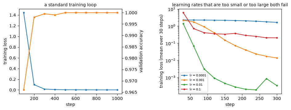
These five lines are the skeleton of all deep learning (nets.train_classifier). Part 2 of script 02 trains SmallCNN on 5000 glyph images; the validation accuracy is 0.966 after 100 steps, 0.998 after 200 and 1.000 after 500. The training loop of a generative model is almost identical; only loss_fn becomes a negative log-likelihood, an ELBO, an adversarial loss or a denoising error.
2.3 Overfitting and the learning rate
Overfitting (part 3 of script 02) uses one MLP with three training-set sizes:
| training images | training accuracy | validation accuracy |
|---|---|---|
| 50 | 1.000 (loss 0.0001) | 0.579 |
| 500 | — | 0.992 |
| 5000 | — | 1.000 |
The 50 images are “memorized” perfectly. For a generative model, overfitting shows up as copying the training set (Lecture 1 §4.5).
Learning rate (part 4 of script 02, Adam, 300 steps):
| learning rate | mean loss of the last 30 steps | validation accuracy |
|---|---|---|
| 1e−4 | 1.665 | 0.675 |
| 1e−3 | 0.0138 | 1.000 |
| 1e−2 | 0.0003 | 1.000 |
| 0.1 | 0.209 | 0.918 |
Too small learns slowly ( is the cross-entropy of guessing); too large is unstable (at 0.1 the loss first shoots above 6). On this easy task 1e−2 is actually fastest — the best learning rate depends on the task and the model, and you have to try. Generative models (especially GANs and large diffusion models) usually need smaller learning rates to stay stable.
2.4 The exponential moving average (EMA) of weights
An EMA maintains a copy of “averaged weights” alongside training:
roughly the average of the weights over the last steps. Part 5 of script 02 uses regression with noisy targets: , batch size only 8, with the true error measured against the noise-free function:
| decay | step | true error of current weights | true error of EMA weights |
|---|---|---|---|
| 0.99 | 500 | 0.108 | 0.048 |
| 0.99 | 1500 | 0.097 | 0.028 |
| 0.99 | 3000 | 0.050 | 0.026 |
| 0.999 | 500 | 0.108 | 0.547 |
| 0.999 | 3000 | 0.050 | 0.039 |
With noisy targets and a small batch, every gradient step is noisy, and the current weights jump around a good solution; the EMA averages the jumps away and is often 2–3× better. A larger decay means a longer window, which lags early in training (it still “remembers” the bad early weights) — the decay must match the training length.
This “regression with noisy targets” is not an arbitrary choice. It is exactly the training target of diffusion models and flow matching, which predict the random noise that was added (Lectures 12, 16). So they almost always sample with EMA weights, with decay often 0.999–0.9999 because they train for hundreds of thousands of steps. (These notes first demonstrated EMA on glyph classification and saw no benefit at all: that task’s loss has no irreducible noise, and the current weights converge well by themselves.)
3. Convolutions, normalization, residuals, U-Net
3.1 Convolutions: local connectivity + weight sharing
A 2-D convolution slides a small kernel (e.g. 3×3) over the image and computes a weighted sum at every position. The output side length is
Part 1 of script 03: 16 kernels of 3×3 (with biases) have only 160 parameters, while a fully connected layer with an output of the same size (16×16×16) needs 1,052,672. A convolution’s parameter count depends only on “kernel size × channels”, not on the image size. That comes from two inductive biases:
- local connectivity: each output looks only at nearby pixels;
- weight sharing: every position uses the same kernel.
A stride-2 convolution halves the side length (downsampling), and a transposed convolution doubles it (upsampling).
3.2 Translation equivariance and receptive fields
Translation equivariance: shift the image by 2 pixels and the conv net’s feature map shifts by 2 pixels. In the code the interior differs by exactly 0; the border differs slightly because of zero padding. The same MLP differs by 0.475. An MLP must learn “digit on the left” and “digit on the right” separately; a convolution does not — which is why convolutions are data-efficient on images.
Receptive field: how large a region of the input one output pixel “can see”.
| 3×3 conv layers | dilation 1 everywhere | 2 everywhere | doubling 1, 2, 4, … |
|---|---|---|---|
| 1 | 3 | 5 | 3 |
| 2 | 5 | 9 | 7 |
| 4 | 9 | 17 | 31 |
| 6 | 13 | 25 | 127 |
Ordinary convolutions grow the receptive field linearly; dilations doubling layer by layer grow it exponentially. That is how WaveNet (Lecture 5) “sees” thousands of audio samples with about 30 layers. PixelCNN (Lecture 6) also needs depth, dilation or downsampling to see far enough.
3.3 Three normalizations: why generative models avoid BatchNorm
Normalization layers “standardize” features (subtract the mean, divide by the standard deviation, then apply a learnable scale and shift), which stabilizes the training of deep networks. They differ in which elements the mean and variance are computed over:
- BatchNorm: per channel, over the whole batch (and all spatial positions);
- LayerNorm: per sample, over all its own channels (and positions);
- GroupNorm: per sample, with the channels split into groups, statistics within each group.
Part 3 of script 03 sends the same sample A through together with two different batches of “companions”. BatchNorm (training mode) changes A’s output by 2.80; LayerNorm and GroupNorm change it by 0. BatchNorm makes a sample’s output depend on who it is processed with. That is a nuisance for generative models:
- a GAN discriminator can use it to “see” that a whole batch is fake;
- when sampling with batch size 1, the statistics are distorted.
So diffusion U-Nets mostly use GroupNorm and Transformers use LayerNorm (nets.TinyUNet and nets.TransformerBlock do the same). In eval mode, BatchNorm switches to running statistics accumulated during training and no longer depends on the companions.
3.4 Residual connections
Without residuals, the gradient is multiplied by a Jacobian at every layer and shrinks exponentially with depth. Part 4 of script 03 (norm of the first layer’s weight gradient at initialization):
| layers | plain network | residual network |
|---|---|---|
| 4 | 1.0e−2 | 2.3e−1 |
| 16 | 8.3e−6 | 1.2e−1 |
| 64 | 9.1e−18 | 5.7e−2 |
The first layer of a 64-layer plain network receives practically no gradient. The residual connection has the Jacobian , which leaves the gradient a “straight-through” path. This is the core idea of the ResNet of Kaiming He et al. (2016); every block of today’s U-Nets and Transformers has a residual.
3.5 The U-Net and time conditioning
The U-Net (Ronneberger et al. 2015) is the standard backbone for “image → image of the same size” tasks:
- the encoder downsamples step by step (smaller side, more channels) to capture global structure;
- the decoder upsamples back to the original size;
- skip connections concatenate the encoder’s features at the same resolution directly into the decoder, preserving high-resolution detail.
Part 5 of script 03 prints the shape after every layer of nets.TinyUNet(ch=16): 16×16×16 → 32×8×8 → 32×4×4 (bottleneck) → 32×8×8 → 16×16×16 → 1×16×16. It has 128,913 parameters in total.
A diffusion model’s denoising network must know “how much noise there is now” (the time or noise level ). The standard recipe:
- Encode the scalar as a vector with a sinusoidal embedding (the same as a Transformer’s positional encoding). Sines and cosines of different frequencies spread nearby values of far apart in some dimensions. Then pass it through a small MLP.
- Use this vector to modulate the features of every residual block with FiLM (Feature-wise Linear Modulation): , one pair per channel. DiT’s adaLN (Lectures 13, 17) is a variant of it.
- Initialize to 0 the linear layer that produces . FiLM then starts as the identity, and the network ignores at first: the code checks that and give identical outputs. Training gradually teaches it to use , and early training is more stable (the same idea as DiT’s “adaLN-Zero”).
The network is then trained for 400 denoising steps: with , input , output the clean image. On 256 new images:
| true noise | the noisy image itself | told | ||
|---|---|---|---|---|
| 0.2 | 0.0400 | 0.0048 | 0.0058 | 0.0064 |
| 0.6 | 0.3603 | 0.0185 | 0.0157 | 0.0160 |
| 1.0 | 1.0010 | 0.0377 | 0.0301 | 0.0287 |
In every row, telling the network the true gives the smallest error; telling it a smaller removes too little noise (clearest in the last row). The network is small and trained for only 400 steps, so the differences are small, but the direction is consistent. This is the seed of the noise-conditional network of Lecture 12: one network, conditioned on the noise level, handles all noise levels.
4. Attention and Transformers
4.1 Scaled dot-product attention
With tokens, each has a query , a key and a value (all linear maps of the input). The -th output is a weighted average of the values, with weights given by the similarity of to each :
Why divide by ? is a sum of products with standard deviation about . Part 1 of script 04 takes :
- without scaling, the scores have std 32 and the softmax is almost one-hot (the largest of 10 weights averages 0.969), so the gradients are tiny;
- divided by , the std is about 1 and the largest weight about 0.32.
So attention stays “soft” for any . The hand-written version differs from PyTorch’s built-in scaled_dot_product_attention by .
The Transformer block (nets.TransformerBlock, pre-norm): ; . Multi-head attention splits the dimensions into subspaces, attends in each and concatenates the results. At one block has about 50,000 parameters (≈ ), independent of the number of tokens — the same Transformer can process sequences of different lengths.
4.2 Permutation equivariance and positional encodings
Neither attention nor the per-token MLP knows “who is where”: shuffle the input and the output is shuffled in the same way (part 2 of script 04: difference ). The order of a sequence or the positions of image patches must be told explicitly. Add a positional encoding (sinusoidal or a learned vector) to every token, and the difference after shuffling becomes 1.884.
Part 5 of script 04 classifies glyphs with a small ViT (a 16×16 image cut into 16 patches of 4×4): 0.9905 with positional encoding, 0.9560 without. Without it the model only sees “which patches are present” — like cutting the image into 16 pieces and shuffling them. The patches’ own shapes (stroke ends, corners, horizontal vs vertical) leak a lot of position information, so it still gets above 90%. To do better, it must know “which patch is where”.
4.3 The causal mask and “shared computation”
In an autoregressive model (Lecture 5), the -th output may depend only on . This is implemented by setting the scores of “future” positions to before the softmax (the causal mask). Part 3 of script 04 adds a random perturbation to token 6:
| attention | change of outputs at positions 0–5 (max) | change at positions 6–9 (min) |
|---|---|---|
| causal mask | 0 | 0.108 |
| no mask | 0.19 | 0.106 |
With the causal mask, changing “the future” has no effect at all on “the past”. More importantly, feeding the whole sequence at once and feeding the first tokens each time and taking the last output give identical results (difference , floating-point error). So when training an autoregressive Transformer, one forward pass yields all conditionals at once — shift the targets by one and this is the “shared computation” of teacher forcing in the Lecture 5 slides. Generation, however, has to go one token at a time.
(An aside: the first version of these notes added 5 to every dimension of token 6, and even “no mask” showed no change at all — LayerNorm subtracts the mean and erased the constant completely.)
4.4 Images become tokens: patchifying
A ViT cuts the image into patches and flattens each into a token (part 4 of script 04):
| patch side | tokens | token dimension | attention matrix size |
|---|---|---|---|
| 1 | 256 | 1 | 65,536 |
| 2 | 64 | 4 | 4,096 |
| 4 | 16 | 16 | 256 |
| 8 | 4 | 64 | 16 |
The cost of attention grows as . With one token per pixel (iGPT’s approach, optional reading in Lecture 7), a 256×256 image has 65,536 tokens and 4.3 billion attention weights. Hence two remedies:
- cut the image into patches;
- or first compress it into a few tokens with a tokenizer (VQ-VAE, VQ-GAN; Lectures 3, 7, 9).
DiT (optional reading in Lecture 13) patchifies in the latent space of a VAE.
5. How to evaluate generative models
5.1 The problem
Lecture 1 §2.5 showed that per-pixel error cannot evaluate generation. Papers on generative models use the following rulers:
- Likelihood / bits/dim (P1 §7): how much probability the model gives test data. Only models that can compute a likelihood can report it: autoregressive models and flows exactly, VAEs and diffusion models as a lower bound.
- FID (Fréchet Inception Distance, Heusel et al. 2017): extract features with a pretrained classifier (the Inception network), fit a Gaussian to the features of real and of generated images, and compute the Fréchet distance between the two Gaussians, . Smaller is better.
- IS (Inception Score, Salimans et al. 2016): — the more confident the classifier on each image and the more even the classes over all images, the higher.
- Precision / recall (Kynkäänniemi et al. 2019): estimate “the manifold of real images” and “the manifold of generated images” with -nearest neighbours in feature space.
- Precision = the fraction of generated images on the real manifold (do they look real?).
- Recall = the fraction of real images on the generated manifold (is the coverage complete?).
5.2 Experiment: seven generators with known defects
The advantage of GlyphWorld is that we can deliberately build “generators” with known defects and see whether each ruler notices. Script 05 replaces Inception with the 64-d features of a SmallCNN trained on glyphs (validation accuracy 0.9995):
| generator | FID ↓ | precision ↑ | recall ↑ | IS ↑ (max 10) | identical to a training image |
|---|---|---|---|---|---|
| (a) fresh real samples | 3.16 | 0.975 | 0.983 | 9.89 | 0% |
| (b) real + noise σ = 0.15 | 56.04 | 0.669 | 0.818 | 9.37 | 0% |
| (c) blurred real | 319.62 | 0.737 | 0.388 | 8.67 | 0% |
| (d) only 0–4 (mode dropping) | 274.21 | 0.979 | 0.494 | 5.00 | 0% |
| (e) copies one training image per digit | 215.05 | 1.000 | 0.000 | 9.95 | 100% |
| (f) one pixel Gaussian per class | 10.10 | 0.467 | 0.940 | 9.10 | 0% |
| (g) one 256-dim pixel Gaussian | 142.62 | 0.104 | 0.802 | 4.77 | 0% |
Reading the table:
- Precision / recall separate “realistic” from “complete”. Mode dropping (d) has precision 0.979 and recall 0.494 (only half the digits); the memorizer (e) has precision 1 and recall 0 (no diversity at all); the pixel Gaussian (g) has precision only 0.104.
- FID folds both into one number, and depends on what the feature extractor cares about. The biggest surprise is (f), the blurry, speckled “one pixel Gaussian per class” samples of Lecture 1 script 03. Their FID is only about 10, “better” than noise (56) or blur (320). In this small classifier’s features a blurry digit is still recognized as that digit, so the feature distribution is close to the real one. Precision (0.467) reveals that more than half its samples do not look real. Real papers’ Inception features are of course richer, but “FID only sees what its feature extractor sees” remains true.
- IS is completely fooled by the memorizer. Copying one training image per digit gives IS = 9.95, above the real samples (every image is a most “typical” digit). IS only asks “is the classifier confident, and are the classes even”, and cannot detect lack of diversity or copying.
- Copying must be checked separately. The last column (the fraction identical to a training image) is the only ruler that directly detects memorization. Real papers check the nearest neighbours of generated images in the training set.
So papers usually report FID together with precision / recall, and show nearest neighbours.
5.3 FID depends on the number of samples
Even with two sets of real images, the FID is not 0 (part 4 of script 05):
| generated samples | 100 | 300 | 1000 | 3000 |
|---|---|---|---|---|
| real vs real FID | ≈ 31.7 | ≈ 15.2 | ≈ 6.6 | ≈ 2.0 |
With few samples the covariance is poorly estimated, and the FID is systematically too large (a biased estimator). Papers usually fix 50,000 samples; FIDs computed with different sample sizes are not comparable.
5.4 Likelihood and sample quality can be completely decoupled
Theis, van den Oord & Bethge (2016) give a simple, powerful argument. Take a good model and build the mixture . Since ,
Spread over dimensions, that is at most bits per dimension. For glyphs, :
- with , the bits/dim gets at most 0.026 worse — only 1.2% relative to the autoregressive table’s 2.134 in P1 — yet 99% of the samples are pure noise;
- with the difference is only 0.052 bits, and 99.99% of the samples are noise.
Conversely, Lecture 1’s “memorizer” (a KDE with a tiny bandwidth) has perfect samples and a test likelihood of .
“High likelihood” and “good samples” are two different things. Autoregressive models and flows report bits/dim; GANs and diffusion models mostly report FID — the two kinds of numbers cannot replace each other.
6. Summary
- Shapes: batch first, images
(N, C, H, W); broadcasting creates bugs that raise no error, so addasserts at key points. Autograd: gradients accumulate, so zero them every step;no_gradis for inference,detachis a stop-gradient. - Reproducibility: set the global seed before building a model, use separate
Generators for data and noise, run single-threaded. Precision: float32 has about 7 significant digits; subtract the maximum before softmax / log-sum-exp. - The training loop is a five-line skeleton. Small data overfits; learning rates must be tried. With noisy targets, the EMA weights are clearly more accurate — exactly the situation of diffusion models.
- Convolutions, normalization, residuals, U-Nets:
- convolutions are local connectivity + weight sharing; they are translation equivariant, and their receptive field grows with depth (exponentially with doubling dilations);
- use GroupNorm / LayerNorm, not BatchNorm;
- residuals make deep networks trainable;
- a U-Net = downsampling + upsampling + skip connections, with the time condition injected through a sinusoidal embedding and FiLM (zero-initialized).
- Attention divides by ; without positional encodings it is permutation equivariant; the causal mask makes one forward pass yield all conditionals (the shared computation of teacher forcing); patchifying controls the cost.
- Evaluation:
- precision / recall separate “realistic” from “complete”;
- FID depends on the feature extractor and on the number of samples;
- IS can be fooled by memorization;
- likelihood and sample quality can be completely decoupled.
7. Common pitfalls
- “The loss goes down, so the code is right.” A broadcasting bug, the wrong BatchNorm mode, targets not shifted by one… all let the loss fall normally while the model learns the wrong thing (§1.1, §3.3, §4.3).
- “I set
torch.manual_seed, so it is reproducible.” Where the seed is set, extra random draws in between and multiple threads all change the results (§1.3). - “EMA always helps.” When the loss has no irreducible noise (e.g. simple classification), the EMA only lags; with a too-large decay it is worse early in training (§2.4).
- “BatchNorm is standard, so generative models should use it too.” It makes samples influence each other; generative models mostly use GroupNorm / LayerNorm (§3.3).
- “Transformers know the order by themselves.” Without positional encodings they are permutation equivariant (§4.2).
- “An autoregressive model must also generate one token at a time during training.” With a causal mask, training is parallel (teacher forcing); only sampling is sequential (§4.3).
- “A low FID means good samples.” FID depends on the feature extractor and may let some defects through; it also depends on the number of samples (§5.2, §5.3).
- “A high IS means a good model.” Memorizing the training set also scores high (§5.2).
- “The higher the likelihood, the better the samples.” The two can be completely decoupled (§5.4).
8. Exercises
Exercise 1 (shapes) The training code of a diffusion model contains x_t = alpha * x0 + sigma * eps, where x0 and eps have shape (N, 1, 16, 16) and alpha, sigma are one number per sample, shape (N,). Does this line raise an error? What is the correct version?
Answer
When broadcasting (N,) against (N, 1, 16, 16), (N,) is treated as (1, 1, 1, N) (shapes are aligned from the last dimension), which clashes with the last dimension 16 — if N ≠ 16 it raises an error; if N happens to be 16, it raises no error but multiplies column i of every image by the i-th sample’s coefficient, the most dangerous case. Correct: alpha[:, None, None, None] * x0 (or alpha.view(-1, 1, 1, 1)), which makes the coefficients (N, 1, 1, 1).
Exercise 2 (convolution shapes) An input of 3×64×64 passes through Conv(3→32, k=3, s=1, p=1) → Conv(32→64, k=4, s=2, p=1) → Conv(64→128, k=4, s=2, p=1) → ConvTranspose(128→64, k=4, s=2, p=1). Write down the output shape after each step and the parameter count of each layer (including biases).
Answer
| layer | output shape | parameters |
|---|---|---|
| Conv(3→32, k=3, s=1, p=1) | 32×64×64 | 3·32·9 + 32 = 896 |
| Conv(32→64, k=4, s=2, p=1) | 64×32×32 | 32·64·16 + 64 = 32,832 |
| Conv(64→128, k=4, s=2, p=1) | 128×16×16 | 64·128·16 + 128 = 131,200 |
| ConvTranspose(128→64, k=4, s=2, p=1) | 64×32×32 | 128·64·16 + 64 = 131,136 |
A transposed convolution’s weight has shape (in channels, out channels, k, k); the count is the same as for an ordinary convolution.
Exercise 3 (the window of an EMA) Show that the EMA weights are a weighted average of all past weights, with coefficient for the weights from steps ago. Why is the “effective window” about ? With , how many steps at least before the EMA has “warmed up”?
Answer
Unroll the recursion: . The coefficients (plus the initial value’s ) sum to 1. The “mean age” of the coefficients is . The weight of the initial value must be small enough (say < 0.05): , about 30,000 steps for . This explains why decay = 0.999 lags for the first few thousand steps in script 02. In practice a “warm-up” decay such as is common.
Exercise 4 (the causal mask) Use nets.attention to write a test verifying that “the -th output has zero gradient with respect to the -th input for ”. Hint: sum one output position, call backward, and look at the input’s .grad.
Answer (sketch)
Let x = torch.randn(1, 8, 16, requires_grad=True), q = k = v = x, out, _ = attention(q, k, v, causal=True); out[0, 3].sum().backward(); check that x.grad[0, 4:] is all zero and x.grad[0, :4] is not. Repeat without causal=True: x.grad[0, 4:] is non-zero. This is the gradient version of “no peeking”.
Exercise 5 (the two Gaussians of FID) Let the two feature sets follow 1-D Gaussians and . Simplify the FID. If the generator outputs a single point () with , what is the FID? Does this mean FID can detect “no diversity”?
Answer
In 1-D, , so FID . With and , FID .
So FID can detect “too little variance” (lack of diversity). But it only compares means and covariances (the first two moments) and cannot see finer structure. Two distributions with the same mean and covariance but completely different shapes have FID 0. The memorizer in script 05 has a large FID (215) because the feature covariance of 10 images is far smaller than the real one.
Exercise 6 (likelihood and samples) A model has 2.0 bits/dim on glyphs. Replace it with the model a uniform distribution (8 bits per pixel). What is the new upper bound on bits/dim? What fraction of samples is uniform noise?
Answer
, i.e. more per dimension: an upper bound of about 2.039 bits/dim. 99.9% of the samples are uniform noise. (The actual value can be slightly lower: the uniform component also contributes a little probability.)
9. Further reading
- C. M. Bishop & H. Bishop, Deep Learning: Foundations and Concepts (2024): Chapters 6–7 (networks and training), 10 (convolutions), 12 (Transformers).
- S. J. D. Prince, Understanding Deep Learning (2023, free online): Chapters 10–12 (convolutions, residuals, Transformers).
- K. He, X. Zhang, S. Ren, J. Sun, Deep Residual Learning for Image Recognition, CVPR 2016.
- O. Ronneberger, P. Fischer, T. Brox, U-Net: Convolutional Networks for Biomedical Image Segmentation, MICCAI 2015.
- Y. Wu & K. He, Group Normalization, ECCV 2018.
- E. Perez et al., FiLM: Visual Reasoning with a General Conditioning Layer, AAAI 2018.
- A. Vaswani et al., Attention Is All You Need, NeurIPS 2017; A. Dosovitskiy et al., An Image is Worth 16x16 Words (ViT), ICLR 2021.
- M. Heusel et al., GANs Trained by a Two Time-Scale Update Rule Converge to a Local Nash Equilibrium (FID), NeurIPS 2017; T. Salimans et al., Improved Techniques for Training GANs (IS), NeurIPS 2016; T. Kynkäänniemi et al., Improved Precision and Recall Metric for Assessing Generative Models, NeurIPS 2019.
- L. Theis, A. van den Oord, M. Bethge, A note on the evaluation of generative models, ICLR 2016.
- MIT6.S184 prerequisite P2:
torch.func(vmap, jacrev), the Hutchinson estimator of divergences, plotting vector fields — used in Lectures 12 and 16. (That course’s notes are in Chinese.)