Maps to: MIT 6.S978 Deep Generative Models (Fall 2024), Reading · Tue 09/24/2024 · Autoregressive (AR) Models (student paper session), plus Problem Set 2 (released 09/24, due 10/08):
- NLL = cross-entropy for binary sequences;
- an unconditional and a class-conditional PixelCNN on MNIST;
- L2 regularization as MAP estimation with a Gaussian prior.
Required papers:
- Y. Bengio & S. Bengio, Modeling High-Dimensional Discrete Data with Multi-Layer Neural Networks, NIPS 1999;
- A. van den Oord, N. Kalchbrenner, K. Kavukcuoglu, Pixel Recurrent Neural Networks, ICML 2016;
- D. P. Kingma, T. Salimans, R. Jozefowicz, X. Chen, I. Sutskever, M. Welling, Improved Variational Inference with Inverse Autoregressive Flow, NIPS 2016.
Basis: This session consisted of student presentations, with no published slides. These notes are organized around the three papers:
- the question they share — “how do we represent the conditionals p(x_i | x_<i) of Lecture 5 well, and what else can the autoregressive structure buy?”;
- each paper’s motivation, method, results and limitations;
- the intermediate models that connect them (NADE, MADE, the Gated PixelCNN of the problem set, MAF).
Numbers from the papers are labelled “the paper reports”. All experiments were designed for these notes and run on a CPU, on binarized GlyphWorld images and the 2-D targets of Lecture 4. Several results contradicted my plan — the most striking: a small VAE beat every autoregressive model here in likelihood. They are reported as they came out. Code:
code/lecture06/— 5 scripts + the shared moduleclassic_ar.py. Each runs in 25–70 s. Reading time: 4–5 hours including running the code.
0. How to read this lecture
0.1 Where we are
Lecture 5 established the recipe: write p(x) = Π_i p(x_i | x_<i), compute all conditionals with one shared network that never looks ahead, train with teacher forcing, sample one variable at a time. It left two questions open:
- How should the conditionals be represented? Lecture 5’s FVSBN gave every pixel its own logistic regression on all previous pixels: simple, exact, and not very good. Better representations share computation and parameters across conditionals and use the 2-D structure of images.
- What else is the autoregressive structure good for? An autoregressive model with Gaussian conditionals is an invertible map with a triangular Jacobian — a normalizing flow (Lecture 4). That flow can make the posterior of a VAE (Lecture 3) richer.
The three papers span seventeen years:
| Paper | Contribution | Descendants |
|---|---|---|
| Bengio & Bengio 1999 | neural networks for the conditionals of high-dimensional discrete data, with shared structure | NADE, MADE |
| van den Oord et al. 2016 (PixelRNN) | deep 2-D architectures for raster-order pixels: Row LSTM, Diagonal BiLSTM, PixelCNN (masked convolutions); a 256-way softmax per sub-pixel | Gated PixelCNN, PixelCNN++, image GPT |
| Kingma et al. 2016 (IAF) | the inverse of an autoregressive flow: one-pass sampling with exact log-density, used as a VAE posterior | MAF, Parallel WaveNet, autoregressive flows in general |
0.2 Learning goals
- Explain the curse of dimensionality for discrete joint distributions, and how the chain rule plus neural conditionals with shared structure avoids it (Bengio & Bengio). Derive NADE’s O(D·H) computation and MADE’s masks.
- Prove that the NLL of a binary autoregressive model equals its binary cross-entropy (Pset 2, problem 1), and that L2 regularization is MAP estimation with a Gaussian prior (problem 4).
- Build masked convolutions of type A and B, explain where each is needed, and what goes wrong otherwise. Find a PixelCNN’s receptive field and its blind spot, and explain how the Gated PixelCNN’s two stacks remove it.
- Condition a PixelCNN on a class (a bias V·y per layer). Measure how much the label is worth in bits, and use the model as a Bayes classifier.
- Explain why an autoregressive model with Gaussian conditionals is a flow, and why MAF evaluates densities in one pass but samples in D passes while IAF does the opposite. Use IAF as a VAE posterior and as a distilled sampler.
- Interpret the experiments: why likelihood and sample quality can disagree, and where global information comes from (receptive field, a condition y, or a latent z).
0.3 Map
| Section | Content | Code |
|---|---|---|
| §1 | Bengio & Bengio; NADE; MADE | 01_nade_made.py part 2 |
| §2 | Problem Set 2: NLL = cross-entropy; weight decay = Gaussian prior | 01_nade_made.py parts 1, 3 |
| §3 | PixelRNN / PixelCNN: masks, blind spot, gated stacks, conditioning | 02_pixelcnn.py, 03_conditional_pixelcnn.py |
| §4 | Autoregressive flows: MAF vs IAF; IAF in a VAE | 04_maf_iaf.py, 05_iaf_vae.py |
| §5 | The big picture | — |
0.4 Data
All image experiments use binarized 16×16 glyphs (gray > 0.5 → 1): 20,000 training images, 2,000 test images, and 5,000 reference images for FID, all with fixed seeds. As in Lecture 5, samples are scored with the Judge’s classifier (“recognizable”: ≥ 90% sure of a digit) and with an FID against binarized real glyphs (held-out real images score 4.3). Likelihoods are teacher-forced NLLs in bits per pixel: a binary pixel costs at most 1 bit, and independent pixels cost 0.413.
1. Neural networks for the conditionals: Bengio & Bengio (1999) and its descendants
1.1 The problem: discrete data in high dimension
Take D binary variables. A full probability table has 2^D − 1 free numbers; the chain rule with full conditional tables has exactly as many (Lecture 5, exercise 1). For D = 256 that is hopeless.
The classical escapes each pay with assumptions:
- naive Bayes / mixtures assume independence given a latent class;
- Bayesian networks restrict each variable to a few parents;
- logistic autoregression (FVSBN) makes every conditional a linear function of all previous variables — O(D²) parameters, but no interactions between parents.
Bengio & Bengio’s proposal is to keep the chain rule and represent each conditional p(z_i | z_1, …, z_{i−1}) with a multi-layer neural network. Its hidden units can represent interactions that a logistic regression cannot, and its connectivity is constrained so that conditional i only sees the variables before i. The paper’s key structural idea is to share the hidden layer’s structure across conditionals rather than train D separate networks, so the parameter count stays manageable while every conditional gets nonlinear features. The paper reports better generalization than simpler models (such as per-variable logistic regressions and naive-Bayes-style models) on several discrete datasets.
This is the template of every later neural autoregressive model: the chain rule for exactness, neural networks for the conditionals, sharing for efficiency.
1.2 NADE: one weight matrix for all conditionals
NADE (Larochelle & Murray 2011) makes the sharing explicit. Conditional i is a one-hidden-layer network on x_<i:
All conditionals share W and c. The pre-activation for position i + 1 is the one for position i plus a single column, a_{i+1} = a_i + W_{:,i} x_i. So all D hidden layers cost O(D·H) together — the same as one hidden layer — instead of O(D²·H). In code it is an exclusive cumulative sum (classic_ar.NADE).
1.3 MADE: masking an ordinary autoencoder
MADE (Germain et al. 2015) gets the same effect from a standard MLP by masking its weights:
- Give each input its position in the chosen order, m(d) ∈ {1, …, D}, and each hidden unit a random “degree” k ∈ {1, …, D − 1}.
- Keep a connection only where information cannot flow from later to earlier:
- input d → hidden k iff k ≥ m(d);
- hidden k → next hidden k′ iff k′ ≥ k;
- hidden k → output d iff m(d) > k (strict, so output d never sees input d).
One ordinary forward pass then gives all D conditionals. Because masks are just numbers, MADE can be trained order-agnostically: draw a new order and connectivity for every minibatch, and at test time average several orders as an ensemble.
1.4 Experiment: FVSBN vs NADE vs MADE
Code 01, part 2 trains all four for 2000 steps on binarized glyphs:
| model | parameters | test bits/pixel | recognizable samples | FID | train time |
|---|---|---|---|---|---|
| FVSBN (no sharing) | 32,896 | 0.1928 | 0.705 | 220.3 | 1 s |
| NADE, H = 128 | 65,920 | 0.1502 | 0.730 | 42.7 | 28 s |
| MADE, 2×500, natural (raster) order | 507,256 | 0.1399 | 0.802 | 52.4 | 2 s |
| MADE, 2×500, 8 random orders (ensemble) | 507,256 | 0.1597 (one order alone 0.1714) | 0.674 | 109.8 | 2 s |
- Sharing a hidden layer pays. NADE and MADE clearly beat FVSBN: the hidden units learn features (“a stroke is coming”, “this is the left edge of a glyph”) that every later conditional reuses.
- Same model class, different computation. NADE grows its pre-activation one column at a time; MADE masks a dense MLP so that one pass gives everything. MADE was about 12× faster per step here, which bought it a much wider network.
- Order matters on images. A single random order is clearly worse than raster order (0.171 vs 0.140): raster order keeps the left and upper neighbours available, as Lecture 5 found for local models. The 8-order ensemble recovers only about a third of the gap. On images, a good fixed order beat order-agnostic training here.
- Samples follow likelihood only roughly. NADE has the lowest FID, MADE the most recognizable digits.
2. Problem Set 2: two short proofs, checked numerically
2.1 Problem 1: NLL equals cross-entropy
For a binary sequence and an autoregressive model with p_i = p(x_i = 1 | x_<i),
Proof. For each i exactly one of y_i, 1 − y_i is 1:
- if x_i = 1, the CE term is −log p_i = −log p(x_i = 1 | x_<i);
- if x_i = 0, it is −log(1 − p_i) = −log p(x_i = 0 | x_<i).
In both cases the term is −log p(x_i | x_<i), the probability of the observed value. Summing over i gives NLL(x) = CE(x). ∎
Code 01, part 1 checks it on 1000 random sequences: the two agree to float rounding.
The practical meaning: training an autoregressive model “like a classifier” with cross-entropy is maximum likelihood. The same holds for softmax outputs over 256 pixel values or 50,000 tokens.
2.2 Problem 4: weight decay is a Gaussian prior
Regularized maximum likelihood maximizes log p(x; θ) − λρ(θ). MAP estimation maximizes the log posterior:
and log p(x) does not depend on θ. So MAP = regularized ML with λρ(θ) = −log p(θ) + const.
For a Gaussian prior θ ~ N(0, σ²I), −log p(θ) = ‖θ‖²/(2σ²) + const. Hence:
L2 regularization with strength λ (penalty λ‖θ‖²) is MAP with a zero-mean Gaussian prior of variance σ² = 1/(2λ).
If the loss is an average over N data points (or N·D pixels, in bits), the data term is scaled by 1/(N·D·ln 2), and the equivalent prior variance becomes σ² = 1/(N·D·ln 2·λ) for Adam’s coupled weight decay, whose gradient term λθ corresponds to the penalty (λ/2)‖θ‖².
Code 01, part 3 trains the 507k-parameter MADE on only 500 images:
| λ | equivalent prior std σ | train bits/pixel | test bits/pixel | gap | ‖θ‖ |
|---|---|---|---|---|---|
| 0 | ∞ (plain ML) | 0.0739 | 0.3326 | +0.259 | 72.6 |
| 1e−5 | 1.06 | 0.0761 | 0.2843 | +0.208 | 55.5 |
| 1e−4 | 0.34 | 0.1140 | 0.2091 | +0.095 | 35.3 |
| 1e−3 | 0.11 | 0.3230 | 0.3317 | +0.009 | 11.9 |
| 1e−2 | 0.03 | 0.4506 | 0.4475 | −0.003 | 5.6 |
Without a prior the model memorizes 500 images: training NLL 0.07, test NLL 0.33. A moderate prior (σ ≈ 0.3) shrinks the weights and cuts the test NLL by a third. A too-narrow prior over-smooths. With 20,000 images (§1.4) the data dominate any reasonable prior.
3. PixelRNN and PixelCNN (van den Oord, Kalchbrenner & Kavukcuoglu 2016)
3.1 Motivation
By 2016, VAEs and GANs produced images but had intractable or unavailable likelihoods. The paper argues for tractable, exact likelihoods — for evaluation, compression and comparison — through the chain rule over pixels, and asks what architecture makes it work on natural images.
Its main ingredients:
- Raster order, sub-pixels in sequence. Pixels are predicted left to right, top to bottom. Within a pixel the colour channels are predicted R, then G given R, then B given R and G, so each “variable” is one 8-bit sub-pixel.
- A discrete 256-way softmax per sub-pixel, instead of a continuous density. The paper reports that it works better than a continuous mixture, because a softmax is free to be multimodal and makes no assumption about the shape of the distribution (Lecture 5 §3).
- Deep 2-D architectures, with residual connections, that compute all conditionals in parallel during training.
3.2 Three architectures
- Row LSTM: an LSTM that processes the image row by row, each row’s state computed by a 1-D convolution from the row above. Its receptive field is a triangle above the pixel; it misses part of the context.
- Diagonal BiLSTM: skews the image so that an LSTM can scan along diagonals in both directions. It gives a receptive field covering all previous pixels — the most expressive of the three, and the slowest.
- PixelCNN: a stack of masked convolutions with no recurrence at all. It is the fastest to train (fully parallel) but has a bounded receptive field.
The paper reports, on CIFAR-10:
| model | bits/dim |
|---|---|
| PixelCNN | 3.14 |
| Row LSTM | 3.07 |
| Diagonal BiLSTM | 3.00 |
These were the best likelihoods on CIFAR-10 at the time. On binarized MNIST the paper reports 79.20 nats with the Diagonal BiLSTM.
3.3 Masked convolutions, type A and B
A k×k convolution sees a square around each pixel. To make it causal, multiply the kernel by a mask:
- keep all rows above the centre;
- in the centre row, keep only the positions left of the centre;
- drop everything below.
There are two variants:
- Type A also hides the centre. In the first layer the centre position is the pixel to be predicted, so it must be hidden.
- Type B keeps the centre. In later layers the centre position holds features that were themselves computed only from earlier pixels, so it is safe, and it lets information flow straight down through the layers.
(With colour, the masks additionally split channels into R/G/B groups so that G may see R at the same pixel but not B.)
5×5 mask A        5×5 mask B
  11111             11111
  11111             11111
  11000             11100
  00000             00000
  00000             00000
Code 02, part 1: with a type-B first layer the model sees the pixel it predicts. The no-peeking test fails before training, and after 300 steps the training loss is 0.0001 bits/pixel instead of 0.152. It is the copy-yourself bug of Lecture 5 §5.2, in two dimensions.
3.4 The blind spot, and the Gated PixelCNN
Which earlier pixels can a stack of masked convolutions actually see? The gradient of one output with respect to the input answers exactly. Code 02, part 2 does this for the output at row 10, column 8:
| network | earlier pixels seen | earlier pixels not seen | later pixels seen |
|---|---|---|---|
| PixelCNN, 5 layers | 126 | 42 | 0 |
| PixelCNN, 12 layers | 158 | 10 | 0 |
| Gated stacks, 5 layers | 75 | 93 | 0 |
| Gated stacks, 12 layers | 168 | 0 | 0 |
PixelCNN, 12 layers        Gated stacks, 12 layers
  ################           ################
  ################           ################
  ...                        ...
  ###############o           ################
  ##############oo           ################
  #############ooo           ################
  ############oooo           ################
  ########X.......           ########X.......
(# = seen, o = earlier but not seen, X = the predicted pixel, . = later pixels.)
-
Both designs are causal: neither ever sees a later pixel.
-
The blind spot. With enough depth the gated stacks see every earlier pixel, but the masked stack keeps missing a wedge up and to the right of the current pixel. A type-B 3×3 kernel at row r reaches row r − 1 only up to column c + 1, and that position’s own features were limited the same way. So the field in the rows just above never grows to the right, however deep the network.
-
The fix. The Gated PixelCNN (van den Oord et al. 2016b, Conditional Image Generation with PixelCNN Decoders — the reference of Problem Set 2) separates the context into two stacks:
- a vertical stack that sees all rows above; its kernel spreads left and right freely, because it never mixes in the current row;
- a horizontal stack that sees the current row to the left, plus the vertical stack’s output.
It also replaces ReLUs by gated activations tanh(W_f ∗ x) ⊙ σ(W_g ∗ x), as in LSTMs. The paper reports that the gated version matches the PixelRNN’s likelihood (about 3.03 bits/dim on CIFAR-10) at PixelCNN’s training speed.
3.5 Experiment: an unconditional PixelCNN (Problem Set 2, problem 2)
Code 02, part 3 trains a small PixelCNN: a 7×7 type-A layer, five residual 3×3 type-B layers, 16 channels and 12,417 parameters, for 1500 steps.
| model | parameters | test bits/pixel | recognizable | FID |
|---|---|---|---|---|
| PixelCNN | 12,417 | 0.1293 | 0.685 | 243.0 |
| MADE, natural order | 507,256 | 0.1399 | 0.802 | 52.4 |
| NADE | 65,920 | 0.1502 | 0.730 | 42.7 |
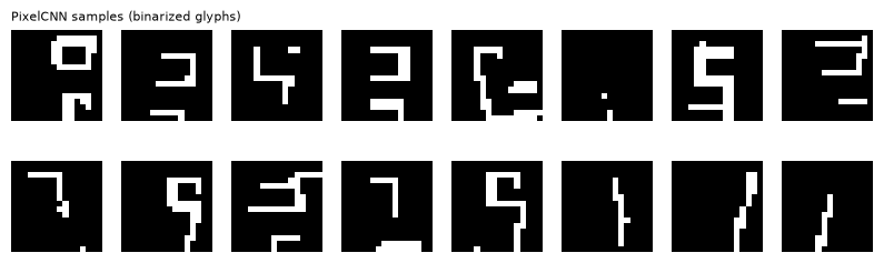
- Likelihood: the best autoregressive model of the lecture, with 40× fewer parameters than MADE. A convolution shares one small local rule across all positions, and for strokes the rows just above and the pixels just to the left are the most informative context.
- Samples: the worst. Strokes are locally plausible, but digits fall apart: segments that do not meet, missing halves, stray bars. With 5 layers each pixel sees only 8 rows up (minus the blind spot), so the bottom of a glyph cannot know which digit its top began. Likelihood averages 256 mostly local predictions; samples need global coherence. This is the same lesson as Lecture 5’s local MLP.
- Sampling speed. With a band trick (compute only the rows a pixel can see), sampling 1000 images takes about 11 s; a full-image recomputation per step would be several times slower.
3.6 Conditioning: p(x | y) (Problem Set 2, problem 3)
To condition on a class label y (one-hot), add a learned class-dependent bias to every masked convolution:
with V_ℓ y broadcast over all pixels. The Gated PixelCNN paper uses the same form for class labels and, with a learned map, for richer conditions such as face embeddings. Code 03 trains it with the same architecture and budget as code 02.
How much is the label worth?
| model | test bits/pixel | bits per image |
|---|---|---|
| unconditional, −log p(x) | 0.1293 | 33.10 |
| conditional, −log p(x | y) | 0.1177 | 30.14 |
The label saves 2.96 bits per image; a label can carry at most log₂ 10 = 3.32. The model uses y almost to the limit. Per pixel that is only 0.013 bits, so conditioning barely moves the bits/dim number.
A generative classifier. argmax_y p(x | y) (Bayes’ rule with a uniform prior, Lecture 1 §3):
- it is 94.1% accurate on test glyphs, although the model was never trained to discriminate;
- its mistakes are between digits that share most strokes (9 → 2, 6 → 5, …);
- mixed back over the labels, log p(x) = log Σ_y p(x | y)/10 gives 0.1294 bits/pixel, exactly the unconditional model’s value. The bits the label saves are, on average, the bits needed to guess the label.
Samples per requested digit:
| samples | recognizable | recognized as the requested digit | FID |
|---|---|---|---|
| unconditional PixelCNN | 0.685 | — | 243.0 |
| conditional PixelCNN | 0.722 | 0.317 | 250.1 |
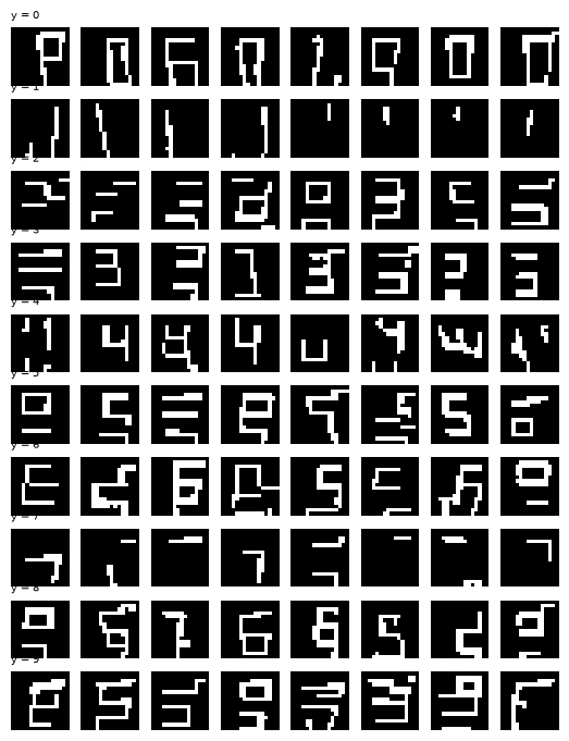
This contradicted my plan. I expected the label — global information available at every pixel — to repair the incoherent samples.
- The label steers strokes, not shapes. The class-specific strokes are clearly there: tall bars for 1, closed boxes for 0, stacked horizontal bars for 3. But only a third of the samples are recognized as the requested digit, and the FID is no better.
- Why prediction and generation differ. In teacher-forced prediction most of the context is given, and the label adds its 3 bits. In free-running sampling the model must compose an entire digit, and a small bias V·y per layer, read through an 8-row receptive field, does not hold the shape together.
- Capacity helps, but not enough. A side check found that more capacity or training (10 layers, 32 channels, or 4000 steps) reaches 0.106–0.112 bits/pixel and 40–46% “as requested”. The problem set’s GPU-trained PixelCNNs on MNIST are much larger. On a CPU budget, likelihood improves long before samples look right.
4. Autoregressive flows: MAF and IAF (Kingma et al. 2016)
4.1 An autoregressive model is a flow
Give every conditional a Gaussian form, x_i = μ_i(x_<i) + exp(α_i(x_<i))·u_i with u_i ~ N(0, 1). This is an invertible map between the noise u and the data x:
- forward: x_i from u_i, given x_<i;
- inverse: u_i = (x_i − μ_i(x_<i))·exp(−α_i(x_<i)).
Its Jacobian ∂x/∂u is triangular, with diagonal exp(α_i), so log|det| = Σ_i α_i. Lecture 4’s change of variables applies: an autoregressive model is a normalizing flow. It is the D-dimensional generalization of the coupling layer (exercise 6).
Which direction is cheap depends on what μ and α are computed from:
| shift and scale depend on | density of a given x | sampling | |
|---|---|---|---|
| MAF (masked autoregressive flow, Papamakarios et al. 2017) | the data x_<i | one pass: all μ_i(x), α_i(x) at once | D passes: x_i needs x_<i |
| IAF (inverse autoregressive flow, Kingma et al. 2016) | the noise u_<i | D passes: recovering u_i needs u_<i | one pass: x = μ(u) + exp(α(u))·u, and log q(x) = log N(u) − Σα for free |
Code 04, part 1 times it, with MADE networks and batch 500:
| D | MAF density | MAF sampling | IAF sampling | IAF density of a given x |
|---|---|---|---|---|
| 8 | 0.2 ms | 1 ms | 0.2 ms | 1 ms |
| 64 | 0.3 ms | 13 ms | 0.5 ms | 13 ms |
| 256 | 0.7 ms | 88 ms | 1.5 ms | 87 ms |
The slow direction is a loop over dimensions and grows with D; at D = 256 it is 60–130× slower. Both directions are exact: recomputing log q of IAF’s own samples the slow way reproduces it to 1e−4.
So MAF suits density estimation, and IAF suits anything that needs fast samples with their own log-density — variational inference, or a fast student. The PixelCNNs of §3 are MAF-like in this sense: fast likelihood, slow sampling.
4.2 Experiments: MAF as a density model, IAF as a sampler
MAF on Lecture 4’s ring of 8 Gaussians (8 layers, maximum likelihood):
| model | KL(p ‖ model) | low-density samples (true 0.010) |
|---|---|---|
| MAF, 8 layers | 0.082 | 0.017 |
| RealNVP, 12 couplings (Lecture 4) | 0.095 | 0.019 |
| i-ResNet, 16 blocks (Lecture 4) | 0.053 | 0.026 |
In 2-D a MAF layer is an affine coupling: x₁’s shift and scale are constants, x₂’s depend on x₁. MAF inherits the coupling flows’ behaviour, bridges between modes included.
Distillation: an IAF student from a MAF teacher. Train an IAF to minimize KL(student ‖ teacher) = E_student[log q(x) − log p_teacher(x)]. The student draws samples and their log q in one pass; the teacher scores them in one pass. This is the idea of Parallel WaveNet (van den Oord et al. 2018), which distilled the slow autoregressive WaveNet into a parallel IAF student for real-time speech.
| model | KL(model ‖ data) | KL(data ‖ model) | low-density | mode shares (ideal 0.125) |
|---|---|---|---|---|
| MAF teacher | 0.129 | 0.082 | 0.017 | 0.118–0.130 |
| IAF student | 1.152 | > 1e3 (modes missing) | 0.012 | 0.000–0.345 |
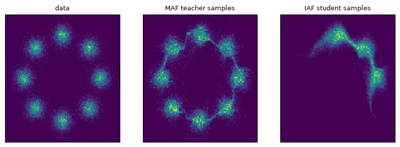
- The student collapsed onto a few modes. KL(student ‖ teacher) only punishes samples where the teacher has little mass; dropping whole modes is cheap — the mode-seeking reverse KL of Lecture 1 §5.3. Its samples are “clean” (few low-density ones), but data from the missing modes have essentially zero density under it.
- Annealing did not help. Annealing the teacher term did not fix it in a check (a mode still had share 0.000).
- Parallel WaveNet needed extra losses (on power spectra, on perceptual features, a contrastive term) for exactly this kind of reason. Fast sampling bought by distillation must be checked for coverage.
IAF for variational inference on two of Lecture 4’s energies (reverse KL, annealed):
| target | IAF, 8 layers | planar flow, 32 layers (Lecture 4) |
|---|---|---|
| U1 | 0.022 | 0.030 |
| U3 | 0.042 | 0.194 |
Each IAF layer reshapes all dimensions with a full triangular Jacobian, not one direction at a time like a planar layer.
4.3 IAF as a VAE posterior
Kingma et al. built IAF for this. The encoder outputs μ, σ and a context vector h; then T IAF steps transform z, each autoregressive in z and conditioned on h:
The gated update (an “LSTM-like” form) is numerically stable. Initialized with σ_t near 1, every step starts close to the identity.
Two points from the paper:
- The IAF lives only in the encoder. Generation (sample z from the prior, decode) costs nothing extra, and in a VAE generation is one pass.
- The paper reports that a ResNet VAE with IAF reached about 3.11 bits/dim on CIFAR-10, close to the PixelCNN family, while sampling orders of magnitude faster.
Code 05: a VAE with a 16-dimensional latent and a Bernoulli decoder, on binarized glyphs, with and without 4 IAF steps. Likelihoods in bits per pixel, the IWAE estimate with K = 512:
| posterior | parameters | −ELBO | −log p(x) (IWAE) | gap | KL term |
|---|---|---|---|---|---|
| diagonal Gaussian | 846,176 | 0.1238 | 0.1127 | 0.0111 | 12.9 nats |
| IAF, 4 steps | 1,004,000 | 0.1248 | 0.1139 | 0.0109 | 12.9 nats |
| samples (1000) | recognizable | FID | time |
|---|---|---|---|
| VAE (diagonal), Bernoulli samples | 0.759 | 80.5 | 1 ms |
| VAE (IAF), Bernoulli samples | 0.796 | 55.7 | 1 ms |
| PixelCNN (§3.5) | 0.685 | 243.0 | ~11 s |
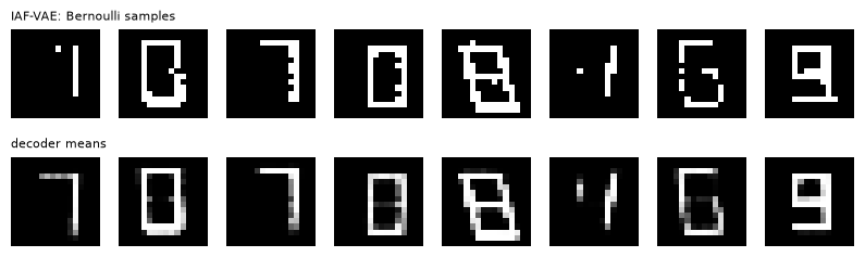
Three results contradicted my plan:
- IAF did not help here. The ELBO and the gap are unchanged; the gap is about 2 nats per image in both. The diagonal Gaussian already leaves little on the table: with a 16-d latent and a strong decoder, the true posterior of these simple images is close to Gaussian. A flexible q pays off when the posterior is far from Gaussian (Lecture 4 §2.4’s bimodal toy); the paper’s gains come from much deeper VAEs on harder data.
- The VAE has the best likelihood of the whole lecture. By its IWAE estimate this small VAE beats every autoregressive model here (0.113 vs PixelCNN 0.129 bits/pixel). The latent captures digit and style; given z, the pixels of a binarized glyph are nearly independent. Our autoregressive models are small CPU models with limited context. On natural images and at scale the ranking usually reverses — but “a VAE always loses on likelihood” is not a law; it depends on how much of the image a latent can explain.
- The VAE’s samples are far better than the PixelCNN’s (FID 56–81 vs 243), and thousands of times faster to draw. Global structure comes from z, exactly what the PixelCNN’s limited receptive field lacked. (Bernoulli samples score a better FID than decoder means because the reference images are binary.)
5. The big picture
5.1 The family tree
chain rule + neural conditionals (Bengio & Bengio 1999)
   ├── FVSBN: one logistic regression per variable (no sharing)
   ├── NADE: one shared hidden layer, cumulative sums             (2011)
   ├── MADE: a masked autoencoder, one pass, any order            (2015)
   │      └── as Gaussian layers → MAF (density) / IAF (sampling, VAE posteriors) (2016-17) → Parallel WaveNet
   └── 2-D architectures for pixels: PixelRNN (Row LSTM, Diagonal BiLSTM), PixelCNN (masked convolutions) (2016)
          └── Gated PixelCNN (no blind spot, conditioning) → PixelCNN++ → image GPT (causal attention, Lecture 5) …
5.2 Where global information comes from
The experiments of this lecture and the last share one theme. Likelihood is a sum of local predictions; samples need a global plan. A model gets global information in one of three ways:
- A large receptive field (Diagonal BiLSTM, gated stacks, attention): every pixel sees all earlier pixels, so the plan emerges from the generated past. This needs depth or attention, and enough capacity to use the context.
- A condition y, given to every position: our class bias carried 3 bits of “which digit” but did not, at this scale, produce coherent digits.
- A latent z drawn first and seen by every pixel (VAE): here the most effective, because 16 numbers describing digit and style are a complete plan for a glyph.
Lecture 7 combines the last two ideas with the first. It first compresses an image into a short sequence of discrete tokens with a learned tokenizer, then models the tokens autoregressively — so each token is a big piece of the image, and the autoregressive model’s context covers the whole image with few steps.
5.3 Compute profiles
| model | likelihood | sampling | architecture constraint |
|---|---|---|---|
| FVSBN / NADE / MADE | exact, 1 pass | D passes | masks / ordering |
| PixelCNN | exact, 1 pass | D passes (H·W·3 for colour) | masked convolutions (blind spot) |
| MAF | exact, 1 pass | D passes per layer | MADE layers |
| IAF | exact for its own samples; D passes for given x | 1 pass | MADE layers |
| VAE (+ IAF posterior) | lower bound; IWAE estimate | 1 decoder pass | none |
6. Summary
- Neural conditionals. Bengio & Bengio (1999) made the template: chain rule for exactness, neural networks for the conditionals, sharing for efficiency.
- NADE shares one weight matrix and computes all hidden layers with a cumulative sum.
- MADE masks an MLP so that one pass gives all conditionals, in any order.
- Sharing beat per-variable logistic regressions clearly; a single random order lost to raster order on images.
- Problem Set 2, problems 1 and 4. Binary cross-entropy is the NLL, so classifier-style training is maximum likelihood. Weight decay λ is a Gaussian prior with σ² = 1/(2λ) in the unnormalized loss. With 500 images it cut the test NLL by a third; too strong a prior over-smoothed.
- PixelCNN. Masked convolutions use type A in the first layer and type B after; a B first layer leaks.
- Stacked masked 3×3 convolutions have a blind spot up and to the right that no depth removes; the Gated PixelCNN’s vertical and horizontal stacks fix it.
- Our small PixelCNN had the best autoregressive likelihood and the worst samples: local context, no global plan.
- Conditioning with a bias V·y per layer used 2.96 of the label’s 3.32 bits and classified 94% of test glyphs correctly by Bayes’ rule. Yet at CPU scale only a third of the samples showed the requested digit.
- Gaussian autoregressive models are flows. MAF evaluates densities in one pass and samples in D; IAF samples in one pass and evaluates given points in D.
- MAF matched coupling flows on the ring.
- An IAF student distilled from MAF by reverse KL dropped modes.
- IAF beat planar flows for VI.
- IAF as a VAE posterior did not help on glyphs, whose posterior is already near-Gaussian. The small VAE itself beat every autoregressive model here in likelihood and samples, by putting the global plan in z.
7. Common pitfalls
- “NADE and MADE are different model classes.” They are two ways to compute the same kind of model (shared nonlinear conditionals): a running sum vs a masked dense pass (§1).
- “Order-agnostic training always helps.” It regularizes and ensembles, but on images a good fixed order can be much better (§1.4).
- “Mask B everywhere is fine.” The first layer must use mask A, or every pixel sees itself (§3.3).
- “A deep enough PixelCNN sees all previous pixels.” Not with stacked masked 3×3 kernels: the blind spot persists (§3.4).
- “Better bits/dim means better samples.” Our PixelCNN had the best autoregressive likelihood and the worst samples (§3.5).
- “Conditioning on the label fixes generation.” It improves likelihood by at most log₂(#classes) bits; turning those bits into coherent samples needs capacity (§3.6).
- “MAF and IAF are the same model.” They are inverses with opposite cost profiles. Using one in its slow direction costs a factor of D (§4.1).
- “Distillation preserves the teacher’s distribution.” Reverse-KL distillation can drop modes (§4.2).
- “A flexible posterior always improves a VAE.” Only if the true posterior is far from the simple family (§4.3).
- “Autoregressive models always beat VAEs on likelihood.” Usually true on natural images at scale, not a law (§4.3).
8. Exercises
Exercise 1 (NADE’s cost). Write the hidden pre-activations a_i = c + Σ_{j<i} W_{:,j} x_j for all i. (a) Show that computing them independently costs O(D²H) and with the recursion a_{i+1} = a_i + W_{:,i}x_i costs O(DH). (b) Count NADE’s parameters for D = 256, H = 128 and compare with FVSBN.
Answer
(a) Independently, a_i needs i − 1 column additions of length H, and Σ_i (i − 1)H = O(D²H). The recursion adds one column per step: O(DH) in total, plus O(DH) for the outputs.
(b) W: H·D = 32,768; V: D·H = 32,768; b: 256; c: 128 — 65,920 in total (matching code 01). FVSBN uses 256·255/2 + 256 = 32,896.
NADE has twice the parameters of FVSBN here, but its hidden units are shared nonlinear features rather than separate linear weights, and its parameter count grows linearly in D, not quadratically.
Exercise 2 (MADE’s masks are correct). With degrees as in §1.3, show that output d depends only on inputs with m(d′) < m(d). Why must the output connection use a strict inequality while the hidden ones do not?
Answer
A path input d′ → h¹_k → h²_{k′} → output d exists only if k ≥ m(d′), k′ ≥ k and m(d) > k′. Chaining gives m(d) > k′ ≥ k ≥ m(d′), so m(d′) < m(d).
The hidden inequalities can be non-strict because hidden units are not variables: a unit of degree k may see inputs up to degree k. The output inequality must be strict, or output d could depend on input d itself (a unit of degree m(d) is allowed to see input d).
Exercise 3 (Problem Set 2, problem 1, general version). Show that for a categorical variable with K values and predicted probabilities p_{i,k}, the NLL equals the categorical cross-entropy −Σ_i Σ_k [x_i = k] log p_{i,k}.
Answer
For each i the one-hot indicator [x_i = k] is 1 for exactly one k, the observed value. So the inner sum equals −log p_{i, x_i} = −log p(x_i | x_<i). Summing over i gives the NLL. The binary case is K = 2 with p_{i,1} = p_i and p_{i,0} = 1 − p_i.
Exercise 4 (Problem Set 2, problem 4). (a) Show that MAP with prior N(μ₀, σ²I) equals regularized ML with penalty ‖θ − μ₀‖²/(2σ²). (b) Which prior corresponds to an L1 penalty λ‖θ‖₁? (c) Code 01’s loss is the mean NLL in bits per pixel over N images of D pixels, plus Adam’s weight decay λ (gradient λθ). Show that the equivalent prior std is σ = 1/√(N·D·ln2·λ).
Answer
(a) log p(θ) = −‖θ − μ₀‖²/(2σ²) + const. Maximizing log p(x | θ) + log p(θ) is maximizing log p(x | θ) − ‖θ − μ₀‖²/(2σ²).
(b) The Laplace prior p(θ) ∝ exp(−λ‖θ‖₁), i.e. each coordinate Laplace with scale 1/λ.
(c) The objective is L = Σ_n NLL_n /(N·D·ln2) + (λ/2)‖θ‖² (the penalty whose gradient is λθ). Multiply by N·D·ln2: Σ_n NLL_n + (N·D·ln2·λ/2)‖θ‖², which is MAP with 1/(2σ²) = N·D·ln2·λ/2, i.e. σ² = 1/(N·D·ln2·λ).
Exercise 5 (the blind spot). For a stack of type-B 3×3 masked convolutions on top of a type-A 3×3 first layer, show by induction that the output at (r, c) never depends on the input at (r − 1, c + 2), however many layers there are.
Answer
Let S_L(r, c) be the set of input positions reachable from the layer-L output at (r, c).
- Base case. The type-A 3×3 layer sees (r−1, c−1), (r−1, c), (r−1, c+1) and (r, c−1).
- Step. A type-B layer at (r, c) combines layer-(L−1) outputs at (r−1, c−1..c+1), (r, c−1) and (r, c), so S_L(r, c) is the union of S_{L−1} at those five positions.
- Claim. Position (r−1, c+2) is never in S_L(r, c). Of the five sources, only (r−1, c+1) could reach it, and S_{L−1}(r−1, c+1) contains only rows ≤ r−1, and in row r−1 only columns ≤ c — the current row of a masked stack only extends left. The other sources are further left or in row r, which never look at row r−1 beyond column c+1 through the same argument.
So the cell (r−1, c+2), and the wedge above it that grows with distance, is never reached.
Exercise 6 (MAF in 2-D is a coupling). Write one MAF layer for D = 2 with order (1, 2), and show it is an affine coupling layer (Lecture 4 §3.1). What does the next layer, with order (2, 1), correspond to?
Answer
x₁ = μ₁ + e^{α₁} u₁ with constants μ₁, α₁ (no predecessors), and x₂ = μ₂(x₁) + e^{α₂(x₁)} u₂. The first coordinate is an affine map with constant parameters (an ActNorm-like scale and shift); the second is scaled and shifted by functions of the first. That is an affine coupling (in the generative direction), plus a per-dimension affine map on x₁.
The reversed-order layer swaps the roles, like alternating coupling masks.
Exercise 7 (IAF’s log-density). For one IAF step z′ = σ ⊙ z + (1 − σ) ⊙ m with (σ, m) computed autoregressively from z, show that log|det ∂z′/∂z| = Σ_i log σ_i. Why does m not appear?
Answer
z′i depends on z_i directly with coefficient σ_i, and on z<i through σ_i and m_i. So ∂z′_i/∂z_j = 0 for j > i, and ∂z′_i/∂z_i = σ_i (σ_i and m_i do not depend on z_i). The Jacobian is lower-triangular with diagonal σ, giving log|det| = Σ log σ_i.
m only affects off-diagonal entries, which do not change a triangular determinant.
Exercise 8 (hands-on).
(a) In 02_pixelcnn.py, replace the five 3×3 layers by ten. Does the sample FID improve as much as the NLL?
(b) In 03_conditional_pixelcnn.py, feed the label also into the input (as 10 extra constant channels). Does “recognized as requested” rise?
(c) In 05_iaf_vae.py, reduce the latent to 2 dimensions. Does IAF help now?
Answer (sketch)
(a) The side check in §3.6 (conditional model) suggests the NLL improves a little and samples improve more slowly. The receptive field grows to 13 rows up, so the plan reaches further, but capacity still limits composition.
(b) Probably slightly. It is equivalent to an extra bias in the first layer, so the effect should be similar to the existing V·y terms. A genuinely stronger form of conditioning (a class embedding that modulates every layer, as FiLM does) is the more likely route.
(c) With a 2-d latent the posterior of an image is often far from Gaussian (several styles can explain a glyph). That is the regime where a flexible q should matter; expect a larger gap for the diagonal posterior and some improvement with IAF. Your run decides.
9. Further reading
The required papers
- Y. Bengio & S. Bengio, Modeling High-Dimensional Discrete Data with Multi-Layer Neural Networks, NIPS 1999.
- A. van den Oord, N. Kalchbrenner, K. Kavukcuoglu, Pixel Recurrent Neural Networks, ICML 2016.
- D. P. Kingma, T. Salimans, R. Jozefowicz, X. Chen, I. Sutskever, M. Welling, Improved Variational Inference with Inverse Autoregressive Flow, NIPS 2016.
Connecting work
- H. Larochelle & I. Murray, The Neural Autoregressive Distribution Estimator, AISTATS 2011 (NADE).
- M. Germain, K. Gregor, I. Murray, H. Larochelle, MADE: Masked Autoencoder for Distribution Estimation, ICML 2015.
- A. van den Oord et al., Conditional Image Generation with PixelCNN Decoders, NeurIPS 2016 (Gated PixelCNN; the problem set’s reference).
- T. Salimans et al., PixelCNN++, ICLR 2017.
- G. Papamakarios, T. Pavlakou, I. Murray, Masked Autoregressive Flow for Density Estimation, NIPS 2017.
- A. van den Oord et al., Parallel WaveNet: Fast High-Fidelity Speech Synthesis, ICML 2018.
- B. Uria et al., Neural Autoregressive Distribution Estimation, JMLR 2016 (a review of the NADE family, including order-agnostic training).
Related notes in this course
- Lecture 5 (the chain rule, teacher forcing, causal architectures, pixel autoregression).
- Lecture 4 §1, §3 (change of variables, coupling layers) and §2.4 (when a flexible posterior helps).
- Lecture 3 §2–§4 (the ELBO, its gap, IWAE).
10. Next lecture
Lecture 7: Tokenizers and autoregressive generation (reading session · 09/26).
This lecture’s pixel models struggled with global structure, because a 16×16 image is 256 small decisions and a local context. Modern autoregressive image generators do not model pixels at all. They first compress an image into a short sequence of discrete tokens with a learned tokenizer (Lecture 3’s VQ-VAE, grown up), then model the tokens with a Transformer. The three papers:
- MAGVIT-v2: lookup-free quantization lets the codebook be huge without its usage collapsing — “the tokenizer is the key”;
- VAR: predict the next scale (a coarse-to-fine pyramid of token maps) instead of the next token;
- TiTok: a 1-D tokenizer that represents an image with as few as 32 tokens.
We will measure codebook usage for VQ, FSQ and LFQ, build a multi-scale residual quantizer, and train small autoregressive models on glyph tokens.