Maps to: MIT 6.S978 Deep Generative Models (Fall 2024), Reading · Thu 10/10/2024 · GAN 2 (student paper session). Required papers:
- N. Huang, A. Gokaslan, V. Kuleshov, J. Tompkin, The GAN is dead; long live the GAN! A Modern GAN Baseline (R3GAN), 2024 (listed on the course page as ICML 2024);
- Z. Wang, H. Zheng, P. He, W. Chen, M. Zhou, Diffusion-GAN: Training GANs with Diffusion, ICLR 2023;
- S. Asokan et al., GANs Settle Scores!, arXiv 2024.
Basis: This session consisted of student presentations, with no published slides. The notes are organized around the session’s question — “what exactly goes wrong in GAN training, and what is the minimal principled fix?” — with three diagnoses: the dynamics (convergence), the signal (non-overlapping distributions), and what the generator’s update means (scores). The background they rely on is explained first: Mescheder et al.’s Dirac-GAN and gradient penalties, instance noise, and the relativistic GAN. Paper claims are labelled “the paper reports / argues”. All experiments were designed for these notes and run on a CPU with 1-D and 2-D toys, where equilibria, divergences and scores are known exactly. Several outcomes were weaker than the papers’ claims at scale, and are reported as they came out:
- the relativistic loss gave no clear gain over R1 on 8 modes;
- Diffusion-GAN’s adaptive noise switched itself off on a 2-D toy.
Code:
code/lecture11/— 4 scripts + the shared modulegan_theory.py. They run in 10–100 s. Reading time: 3–4 hours including running the code.
0. How to read this lecture
0.1 Where we are
Lecture 9 listed the problems of GANs — oscillation, vanishing gradients, mode collapse — and Lecture 10 showed large GANs that work, held together by a stack of stabilizers: R1 penalties, pretrained discriminator features, careful architectures. This session asks what is actually wrong, and gives three complementary answers:
| diagnosis | question | paper | fix |
|---|---|---|---|
| dynamics | Does gradient descent on the min–max game converge to the equilibrium at all? | R3GAN (building on Mescheder et al. 2018) | a relativistic loss with R1 + R2 gradient penalties, provably locally convergent |
| signal | Does the discriminator’s gradient carry information when the two distributions do not overlap? | Diffusion-GAN (building on instance noise) | noise both distributions with a forward diffusion so they always overlap |
| meaning | What does the generator’s update do, in terms of the two densities? | GANs Settle Scores! | it moves samples along a (smoothed) difference of score functions, linking GANs to score matching and diffusion |
0.2 Learning goals
- Analyze the Dirac-GAN: compute the Jacobian of the training dynamics, explain why purely imaginary eigenvalues mean no convergence, and show how R1 / R2 or instance noise fix it.
- Explain the relativistic pairing loss (RpGAN), why it is argued to remove mode-dropping local minima, and R3GAN’s claim that RpGAN + R1 + R2 makes the old tricks unnecessary.
- Explain Diffusion-GAN: forward-diffusion instance noise on real and fake samples, a timestep-aware discriminator, the adaptive noise level, and why noise makes non-overlapping distributions learnable.
- Derive that the optimal discriminator’s gradient is the difference of the data’s and the generator’s scores, and explain the “smoothed score matching” reading of IPM GANs.
- Connect all three to Lecture 12: scores, noise levels, and moving samples along gradients.
0.3 Map
| Section | Content | Code |
|---|---|---|
| §1 | Three diagnoses | — |
| §2 | Convergence: the Dirac-GAN and gradient penalties | 01_dirac_gan.py |
| §3 | R3GAN: a relativistic loss with R1 + R2 | 02_r3gan_loss.py |
| §4 | Diffusion-GAN: instance noise from a forward diffusion | 03_instance_noise.py |
| §5 | GANs settle scores | 04_score_difference.py |
| §6 | The big picture | — |
1. Three diagnoses of an unhealthy game
Recall the game (Lecture 9): . The theory says the unique equilibrium is with . Three gaps separate that statement from practice:
- Existence is not convergence. An equilibrium may exist, and simultaneous or alternating gradient steps may still circle around it forever. This is a property of the dynamics, studied with the eigenvalues of the update map near the equilibrium.
- A good discriminator can be useless. When and do not overlap — the typical case for images — a strong D separates them perfectly. JS is stuck at log 2 and the saturating G-loss has no gradient (Lecture 9 §5.1).
- The landscape can have traps. Even with good dynamics, the generator’s loss as a function of its parameters may have bad local minima. Configurations that drop modes are the classic example.
2. Convergence: the Dirac-GAN and gradient penalties
2.1 The smallest GAN
Mescheder, Geiger & Nowozin (2018) strip a GAN down to two scalars:
- the data are a point mass at 0;
- the generator is a point mass at θ;
- the discriminator is linear, (a logit).
The equilibrium is (θ, ψ) = (0, 0): the generator on the data, and a flat discriminator.
With the non-saturating loss the real logit is and the fake logit is ψθ:
Gradient descent follows the vector field :
At (0, 0), with σ(0) = ½, the Jacobian and its eigenvalues are
Purely imaginary eigenvalues: a rotation. Read the dynamics as a story:
- the generator sits at θ > 0;
- D tilts its line to reject it;
- G slides down the tilt, past 0;
- D tilts the other way, and so on.
Continuous-time gradient flow circles forever. Discrete steps make it worse: simultaneous updates multiply the radius by per step near the equilibrium, while alternating updates are neutral to first order.
2.2 Fixes: penalties and noise
R1 penalizes the discriminator’s gradient on real data, ; R2 does the same on fake data. For the linear D both equal , which adds to ψ’s update:
Both eigenvalues now have real part −γ/2 < 0 (for γ < 1, , a damped spiral). The equilibrium is locally convergent.
Why doesn’t the penalty move the equilibrium? At the optimal D is constant, so and the penalty costs nothing there. It only discourages D from being steep at the data, which is exactly what drove the rotation.
Instance noise (Sønderby et al. 2017; Arjovsky & Bottou 2017) adds noise to both real and fake samples before D sees them. The losses become expectations over the noise, and their curvature in ψ acts like a penalty: the eigenvalues get negative real parts too.
Mescheder et al. also show that the unregularized loss, WGAN with clipping and, in general, WGAN-GP are not locally convergent in this sense.
2.3 Experiment: the Dirac-GAN, numerically
Code 01 runs gradient descent from (θ, ψ) = (1, 1) with step size 0.1. Distance to the equilibrium:
| loss / regularizer | simultaneous: @1000 | @3000 | steps to < 0.01 | alternating: @1000 | @3000 | steps to < 0.01 |
|---|---|---|---|---|---|---|
| standard (non-saturating) | 0.467 | 0.447 | never | 0.281 | 0.163 | never |
| relativistic (RpGAN) | 0.467 | 0.447 | never | 0.281 | 0.163 | never |
| WGAN, clipping ±1 | 1.072 | 1.000 | never | 1.005 | 0.975 | never |
| standard + R1, γ = 1 | 0 | 0 | 153 | 0 | 0 | 158 |
| standard + R1, γ = 0.1 | 0.015 | 0 | 1120 | 0.005 | 0 | 865 |
| standard + instance noise σ = 0.7 | 0 | 0 | 427 | 0 | 0 | 376 |
| RpGAN + R1 + R2 (γ = 0.5 each) | 0 | 0 | 153 | 0 | 0 | 158 |
The eigenvalues computed numerically at (0, 0):
| loss | eigenvalues |
|---|---|
| standard / RpGAN | ±0.500i |
| + R1, γ = 1 | −0.500 (double) |
| + R1, γ = 0.1 | −0.050 ± 0.497i |
| + instance noise σ = 0.7 | −0.122 ± 0.485i |
| RpGAN + R1 + R2 | −0.500 (double) |
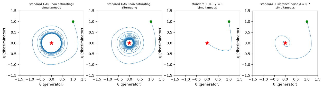
- The unregularized game never settles. With simultaneous steps it ends on a cycle of radius ~0.45, reached from outside and from inside: started at radius 0.14 it moved out to 0.45. The linear analysis predicts outward spiralling, and the loss’s nonlinearity stops it at a finite radius. Alternating steps creep inward sublinearly (radius 0.06 after 20,000 steps).
- Penalties and noise converge. They are fast when the damping is strong (γ = 1: 153 steps) and slow when it is weak (γ = 0.1: about 1000).
- In the Dirac-GAN, RpGAN is identical to the standard loss, because the real logit is always 0. Its advantages, if any, lie elsewhere (§3).
On WGAN-GP. With a one-parameter linear critic, WGAN-GP’s penalty has a kink at ψ = 0. In development, gradient descent stalled there with the generator at θ = 2 — an artifact of the toy, so it is left out of the table.
3. R3GAN: a well-behaved loss with no tricks
3.1 The claim
R3GAN’s abstract argues against the widespread belief that GANs are inherently hard to train:
- derive a well-behaved regularized relativistic GAN loss that addresses mode dropping and non-convergence — problems previously tackled with a bag of ad-hoc tricks;
- prove that it is locally convergent, unlike most relativistic losses;
- then discard the tricks and replace StyleGAN2’s outdated backbone with a modern one.
The resulting minimalist baseline, R3GAN, is reported to surpass StyleGAN2 on FFHQ, ImageNet, CIFAR and Stacked MNIST, and to compare favourably with state-of-the-art GANs and diffusion models.
3.2 The relativistic pairing loss
The standard discriminator judges each sample in absolute terms: real or fake? The relativistic pairing GAN (RpGAN, Jolicoeur-Martineau 2019) judges pairs: is this real sample more real than this fake one?
Why should that help with mode dropping? R3GAN builds on Sun et al. (2020), who analyze the generator’s loss landscape (with the discriminator at its optimum) over configurations of generated points:
- for the standard GAN, configurations in which generated points pile onto a subset of the data modes are bad local minima — exponentially many of them;
- for RpGAN every basin is global.
Intuitively, the standard D can be satisfied by labelling each sample on its own, so a generator that covers some modes perfectly is “locally fine”. RpGAN’s comparisons couple every fake with every real sample, so missing modes keep producing pairs that the generator can improve.
3.3 Making it converge: R1 + R2
RpGAN alone inherits the rotation of §2: in the Dirac-GAN it is identical to the standard loss. R3GAN adds both R1 (gradient penalty on real data) and R2 (on fake data), and proves local convergence for the combination. It reports that leaving out a penalty leads to training failures.
3.4 The roadmap: from StyleGAN2 to R3GAN
With a loss that is well behaved by itself, the paper strips StyleGAN2 step by step:
- Removed tricks: the mapping network and style injection, mixing regularization, path-length regularization, minibatch standard deviation, lazy regularization and others.
- New backbone: a modern convolutional design in place of the 2019 one — ResNet-style residual blocks modernized in the ConvNeXt manner, with grouped convolutions and inverted bottlenecks, no normalization layers, and careful initialization.
The paper reports that the simplified, modernized model trains stably and beats StyleGAN2. It also reports full coverage of the 1000 modes of Stacked MNIST, a standard mode-dropping test.
3.5 Experiment: losses on the 8-mode ring
Code 02 trains Lecture 9’s MLP GAN on the narrow 8-mode ring with four seeds per loss (5000 steps). “Drift” measures how much the mix of modes changes every 500 steps late in training.
| loss | modes covered (seeds 0–3) | mean modes | mean quality | drift |
|---|---|---|---|---|
| standard (non-saturating) | 4 / 3 / 4 / 7 | 4.50 | 0.902 | 0.120 |
| standard + R1 (γ = 1) | 8 / 8 / 8 / 8 | 8.00 | 0.897 | 0.114 |
| relativistic, no penalty | 6 / 4 / 4 / 8 | 5.50 | 0.922 | 0.119 |
| RpGAN + R1 + R2 (γ = 1 each) | 8 / 6 / 8 / 8 | 7.50 | 0.822 | 0.187 |
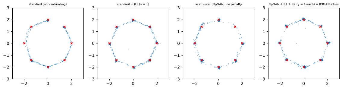
- R1 is the decisive ingredient at this scale: all 8 modes in all four seeds. It fixes coverage but not motion: the drift barely changes, so the mix of modes keeps shifting by ~11% every 500 steps. With a finite learning rate the iterates keep moving near the equilibrium; §2’s damped spiral describes small steps close to it.
- The relativistic loss alone helps a little (5.5 vs 4.5 modes).
- The full R3GAN loss at γ = 1 each was slightly worse than standard + R1, with lower quality and more drift. The R2 penalty on fakes, at this weight, slows the generator down. R3GAN tunes γ per dataset; we did not.
Development note. On the 25-mode grid the outcomes varied too much between seeds to rank the losses: standard + R1 + R2 covered 8 modes with one seed and 23 with another. On 8 modes we confirm that the gradient penalties — the part of R3GAN that carries its convergence proof — make the difference. The benefit it reports for the relativistic part, on data with ~1000 modes and on real images, is not visible at this scale.
4. Diffusion-GAN: instance noise from a forward diffusion
4.1 The problem, again
Real images occupy a thin, low-dimensional set in pixel space; so do generated ones; two such sets typically do not intersect (Arjovsky & Bottou 2017). Then:
- the optimal D separates them perfectly, JS = log 2 regardless of their distance, and the saturating loss has no gradient (Lecture 9);
- a strong D overfits the finite training set — a growing problem with limited data.
Instance noise is the classic fix. Add the same kind of noise to real and fake samples, so that the noised distributions and have full support and always overlap. In practice a single noise level is hard to choose: too little does nothing, too much hides everything.
4.2 Method
Diffusion-GAN replaces the single level by a forward diffusion chain (Lecture 12):
- Noising. For a sample x (real or fake) and a level t ∈ {0, …, T}: . Real and fake samples are noised the same way, with t drawn from a distribution over {0, …, T}.
- A timestep-dependent discriminator learns to discriminate at every noise level: easy and informative at high noise, sharp at low noise.
- Gradients through the noise. The generator receives gradients through the noising, which is a reparameterized, differentiable function of G(z). It is trained to match the data at all noise levels at once.
- Adaptive T. The paper monitors , i.e. how confidently D recognizes real samples. If exceeds a target, D is overfitting, so T increases (more noise); otherwise T decreases.
Theory (the paper’s two points).
- With the noise, the objective is continuous and differentiable in the generator’s parameters even when the clean distributions do not overlap.
- Matching the noised distributions at a level t implies matching the clean ones, because convolution with a Gaussian is invertible on distributions. So the noise does not change what is learned, only how well the signal flows.
Results. It reports improvements over strong GAN baselines (StyleGAN2, Projected GAN, InsGen) on a range of image datasets. It also points out that the diffusion noise acts as a domain-agnostic, differentiable augmentation.
4.3 Experiment: noise makes a far-away generator learnable
JS between noised point masses (code 01, part 1): N(0, σ²) vs N(θ, σ²).
| σ | θ = 0.25 | 0.5 | 1 | 2 | 4 | 8 |
|---|---|---|---|---|---|---|
| 0 (point masses) | 0.6931 | 0.6931 | 0.6931 | 0.6931 | 0.6931 | 0.6931 |
| 0.1 | 0.4417 | 0.6759 | 0.6931 | 0.6931 | 0.6931 | 0.6931 |
| 0.5 | 0.0303 | 0.1114 | 0.3368 | 0.6327 | 0.6931 | 0.6931 |
| 1.0 | 0.0078 | 0.0303 | 0.1114 | 0.3368 | 0.6327 | 0.6931 |
| 2.0 | 0.0019 | 0.0078 | 0.0303 | 0.1114 | 0.3368 | 0.6327 |
The noise turns a flat JS into a smooth function of θ. Its useful range grows with σ — the reason for using many levels.
A spike chasing a spike (part 2). The data are N(0, 0.05²); the generator is θ + 0.05ε, starting at θ = 4; the discriminator is strong (5 D-steps per G-step). θ after training:
| instance noise | G-loss | θ @100 | @300 | @1500 |
|---|---|---|---|---|
| none | minimax | 3.972 | 3.971 | 3.971 |
| none | non-saturating | 0.000 | −0.001 | −0.006 |
| σ = 0.3 | minimax | 3.967 | 3.965 | 3.964 |
| σ = 1.0 | minimax | 3.031 | 0.094 | −0.003 |
| σ = 2.0 | minimax | 2.880 | 1.039 | 0.004 |
| σ = 2.0, annealed to 0 | minimax | 2.826 | 0.583 | −0.002 |
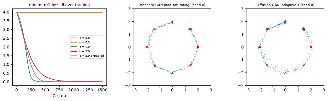
- With the original minimax loss and little noise, the generator never moves. D separates the spikes, D(G(z)) ≈ 0, and log(1 − D) is flat there.
- With σ ≥ 1, the same loss pulls θ to the data. Annealing keeps the early signal and ends noise-free.
- The non-saturating loss reaches the data without noise. Our MLP discriminator’s logit keeps sloping beyond the data (LeakyReLU extrapolates linearly), so −log D still has a gradient. Noise is what makes the saturating objective, and JS itself, informative.
Diffusion-GAN on the 8-mode ring (part 3, three seeds):
| model | modes covered | quality |
|---|---|---|
| standard GAN | 4 / 3 / 4 | 0.90 / 0.86 / 0.92 |
| Diffusion-GAN, adaptive T | 4 / 6 / 3 | 0.89 / 0.94 / 0.59 |
The adaptive rule turned the noise down to its minimum (T = 1). D never classified real samples confidently enough to trigger more noise. Diffusion-GAN reduced itself to a plain GAN with a time-conditioned D, and varied between seeds like the standard GAN. In 2-D the generator’s samples overlap the data quickly, so the problem instance noise addresses hardly arises. Part 2 isolates the mechanism; the paper’s gains are on images.
5. GANs settle scores
5.1 The discriminator’s gradient is a score difference
For a fixed generator, the optimal discriminator is (Lecture 9). Its logit is the log density ratio:
so its gradient is a difference of score functions (, Lecture 12):
The non-saturating G-step moves each generated sample up the discriminator’s logit:
So each sample is pushed toward higher data density and away from where the generator already over-produces, weighted by how fake it still looks. The generator stops moving when wherever it puts mass: a score-matching condition.
5.2 The paper’s unified view
Asokan et al. analyze the generator’s optimization variationally, treating it as an optimization over the generator’s output distribution rather than over the discriminator:
- f-divergence GANs. The optimal generator matches the score of its output distribution to the score of the data. The standard GAN is one f-GAN.
- IPM GANs (Wasserstein with Lipschitz or gradient constraints, MMD). The optimal generator matches score-like functions involving the kernel associated with the constraint. The paper reads this as smoothed score matching: the scores of the data and of the generator are convolved with that kernel.
From this view the paper proposes alternatives to GAN training based on score and flow matching, and discriminator-guided Langevin sampling. It also offers explanations for empirical observations, such as the stability of the non-saturating loss.
5.3 Experiment: checking the gradients, and a GAN without a generator
Code 04 trains a logistic discriminator and a WGAN-GP critic between 8 Gaussians of std 0.2 on a ring and . Both scores are known exactly. It compares the gradients at 4000 points with the exact score difference, and with differences of scores smoothed by N(0, h²):
| discriminator | cosine, mean | cosine, median | vs smoothed h = 0.25 | h = 0.5 | h = 1 | corr(output, log ratio) |
|---|---|---|---|---|---|---|
| logistic (standard GAN) | 0.963 | 0.992 | 0.937 | 0.744 | 0.290 | 0.934 |
| WGAN-GP critic | 0.839 | 0.958 | 0.874 | 0.782 | 0.432 | 0.924 |
- The logistic discriminator’s gradient is the score difference, almost everywhere.
- The WGAN-GP critic’s gradient aligns best with a mildly smoothed score difference (h = 0.25), in line with the smoothed-score-matching reading. Its magnitude is fixed by the penalty (≈ 1), not by the densities.
Moving particles along the discriminator’s gradient (part 2). Start 2000 particles from . Each round, update D for 5 logistic-regression steps (real = data, fake = particles), then move every particle by . There is no generator network at all.
| data | modes covered | quality | mode entropy | time |
|---|---|---|---|---|
| ring, std 0.2 | 8 | 0.988 | 3.00 | 1.1 s |
| ring, std 0.05 | 8 | 0.980 | 3.00 | 1.1 s |
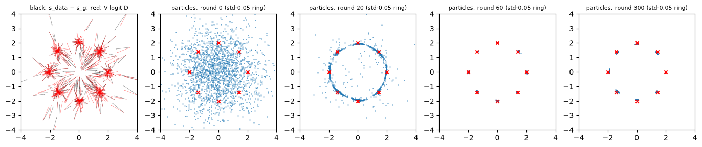
On exactly the narrow ring where Lecture 9’s generator network covered 3 of 8 modes, the particles reach all 8, balanced. The discriminator’s signal, , points toward the missing modes. What failed in Lecture 9 is a generator network that must realize all these moves with one shared set of weights, in a game played by alternating gradient steps.
This is the bridge to Lecture 12. Moving samples along a score is what Langevin dynamics and diffusion samplers do, with the score learned by denoising instead of by a discriminator.
6. The big picture
6.1 Three views of one game
| view | object of study | failure | principled fix | our evidence |
|---|---|---|---|---|
| dynamics | eigenvalues of the update at the equilibrium | rotation (±i/2) → cycles | R1 / R2 penalties, instance noise | Dirac-GAN converges only with them; R1 gave 8/8 modes in all seeds |
| signal | divergence between non-overlapping distributions | JS constant, saturating gradients | noise both distributions (Diffusion-GAN) | the minimax loss moves only with σ ≥ 1 |
| meaning | the generator’s update direction | — | read it as score difference (f-GANs) or smoothed score difference (IPM GANs) | cosine 0.99 (logistic), 0.87 to smoothed scores (WGAN-GP); particles cover all modes |
6.2 What this means for the rest of the course
- Noise levels (Diffusion-GAN) and scores (GANs Settle Scores) are exactly the ingredients of diffusion models.
- Lecture 12 starts from energy-based models and score matching: learn directly, by denoising, and generate by moving samples along it — no adversary, no rotation.
- The price is many steps per sample, which Lectures 13 and 18 then try to remove. A circle back to Lecture 10’s distillation into GANs.
7. Summary
- Convergence. In the Dirac-GAN the unregularized game has eigenvalues ±i/2: the players rotate around the equilibrium. Our runs ended on a cycle (simultaneous steps) or crept in sublinearly (alternating). R1 / R2 penalties add damping, λ = (−γ ± √(γ² − 1))/2, and instance noise also damps; both converge.
- R3GAN. Relativistic pairing (argued to remove mode-dropping minima) plus R1 + R2 (locally convergent) makes the old tricks unnecessary and supports a modern backbone. On 8 modes, R1 alone did the decisive work; the relativistic part’s benefit was not visible at our scale.
- Diffusion-GAN. Noise real and fake samples by a forward diffusion with an adaptive maximum level; D sees the level; G is trained through the noise. Noise makes JS smooth and revived a stuck minimax-loss generator; on a 2-D toy the adaptive schedule switched the noise off.
- Scores. The optimal discriminator’s logit is the log density ratio, so its gradient is . GAN generators perform (smoothed) score matching. Particles moved along a trained discriminator’s gradient covered every mode where a generator network collapsed.
8. Common pitfalls
- “An equilibrium exists, so training converges.” Existence says nothing about the dynamics; the plain game rotates (§2).
- “Gradient penalties change what the GAN learns.” At the equilibrium D is constant and the penalty is zero; they change only the dynamics (§2.2).
- “R1 freezes the game.” It damps the rotation near the equilibrium; with finite steps, samples keep drifting (§3.5).
- “Instance noise blurs the results.” Matching noised distributions implies matching clean ones; and noise can be annealed (§4.2–4.3).
- “The relativistic loss is a convergence fix.” Alone it is not (identical to the standard loss in the Dirac-GAN); its argued benefit is the landscape, and convergence comes from R1 + R2 (§3).
- “Mode collapse means the discriminator gives bad directions.” The discriminator’s gradient is a score difference that points at missing modes; collapse comes from how a generator network and alternating steps follow it (§5.3).
9. Exercises
Exercise 1 (Dirac-GAN eigenvalues). For the minimax G-loss (instead of the non-saturating one), compute the Jacobian at (0, 0). Does the flip trick change the local dynamics?
Answer
, so . Its derivatives at 0 are and . The D part is unchanged.
So J is identical, with eigenvalues ±i/2. The flip trick changes the dynamics far from the equilibrium (gradient strength when D rejects fakes, Lecture 9 §2.2), not the local rotation.
Exercise 2 (RpGAN = standard GAN in the Dirac-GAN). Show that the RpGAN losses of §3.2 coincide with the non-saturating standard losses when the data are a point mass at 0 and D is linear. Why does this make the Dirac-GAN unable to show RpGAN’s advantage?
Answer
, so .
- , which equals the standard D-loss minus the constant softplus(0).
- , the non-saturating G-loss.
RpGAN’s argued benefit is about the landscape with many data modes (generated points coupled to every real point). A single data point has no modes to drop, so the Dirac-GAN tests only the local dynamics, which are identical.
Exercise 3 (why penalties don’t move the optimum). Show that if , the D maximizing (over logits) is constant, so the regularized game has the same equilibrium.
Answer
With :
maximized pointwise by a = 0, with value −log 4.
A constant a = 0 has zero gradient, so the penalty is 0 too. Any non-constant a lowers V and pays a non-negative penalty, so a ≡ 0 remains optimal. The generator, facing a flat D, receives no gradient: the equilibrium is unchanged.
Exercise 4 (noise and overlap). Let and in 1-D. (a) Compute . (b) Show it is differentiable in θ, while JS(p ‖ q) is not. (c) Why can Diffusion-GAN claim that matching noised distributions implies matching clean ones?
Answer
(a) The KL between N(0, σ²) and N(θ, σ²) is θ²/(2σ²).
(b) This is smooth in θ, with gradient θ/σ². JS(δ₀ ‖ δ_θ) is log 2 for θ ≠ 0 and 0 at θ = 0: discontinuous, with zero gradient almost everywhere.
(c) Convolution with a Gaussian multiplies characteristic functions by , which is never zero. So equal noised characteristic functions imply equal clean ones: the noised distributions determine the clean ones. For the diffusion noise , rescaling by is also invertible.
Exercise 5 (the generator’s update as a score difference). Starting from and with , derive the expression of §5.1. What changes for the minimax G-loss?
Answer
Non-saturating loss. has derivative with respect to a. By the chain rule,
Minimax loss. has derivative , so the weight becomes . The direction is the same score difference, weighted by D(x) instead of 1 − D(x). This vanishes exactly for samples that D confidently calls fake: the saturation of Lecture 9, now in score language.
Exercise 6 (hands-on).
(a) In 01_dirac_gan.py, add a two-time-scale variant (the discriminator’s step 10× larger than the generator’s). Does the unregularized game converge?
(b) In 02_r3gan_loss.py, try RpGAN + R1 + R2 with γ = 0.1 each. Does quality recover?
(c) In 04_score_difference.py, replace the moves by (i) pure gradient ascent on the exact data score, , and (ii) Langevin dynamics, . Compare both with the discriminator-guided flow.
Answer (sketch)
(a) Different time scales change the eigenvalues of the discrete map, but without damping the continuous dynamics still rotate. Expect cycles or slow convergence, not the fast convergence of R1.
(b) A weaker R2 slows the generator less. Development runs on the grid showed outcomes are very seed-dependent, so compare several seeds.
(c) Pure ascent on drives every particle to a mode centre: zero spread, a point-mass caricature of the data. Langevin dynamics adds exactly enough noise for its stationary distribution to be — Lecture 12’s sampler. The discriminator-guided flow needs no noise because its drift is a difference : the term pushes particles apart where they crowd, and the flow stops when . The repulsion that Langevin gets from noise, the GAN gets from the generator’s own score.
10. Further reading
The required papers
- N. Huang, A. Gokaslan, V. Kuleshov, J. Tompkin, The GAN is dead; long live the GAN! A Modern GAN Baseline, 2024.
- Z. Wang, H. Zheng, P. He, W. Chen, M. Zhou, Diffusion-GAN: Training GANs with Diffusion, ICLR 2023.
- S. Asokan et al., GANs Settle Scores!, arXiv 2024.
Background
- L. Mescheder, A. Geiger, S. Nowozin, Which Training Methods for GANs do actually Converge?, ICML 2018 (the Dirac-GAN, R1 / R2).
- A. Jolicoeur-Martineau, The relativistic discriminator: a key element missing from standard GAN, ICLR 2019.
- R. Sun, T. Fang, A. Schwing, Towards a Better Global Loss Landscape of GANs, NeurIPS 2020.
- C. K. Sønderby et al., Amortised MAP Inference for Image Super-resolution, ICLR 2017 (instance noise).
- M. Arjovsky, L. Bottou, Towards Principled Methods for Training Generative Adversarial Networks, ICLR 2017.
- S. Nowozin, B. Cseke, R. Tomioka, f-GAN, NeurIPS 2016.
Related notes in this course
- Lecture 9 (the game, D*, JS, mode collapse); Lecture 10 §2 (R1 in StyleGAN).
- P1 (KL, convolution with Gaussians).
11. Next lecture
Lecture 12: Energy-based models, score matching and diffusion models (lecture · 10/17, with Problem Set 4).
This lecture ended with samples moving along a score difference supplied by a discriminator. Lecture 12 removes the discriminator and learns the score of the data directly:
- energy-based models write and never need the normalizing constant for the score;
- score matching and denoising score matching learn by predicting the noise added to data;
- Langevin dynamics samples with the score;
- diffusion models chain many noise levels — the levels Diffusion-GAN used — into a generative model whose training objective is a simple L2 regression.